Breaking the Token Ceiling: Distilling Smaller, Stronger Byte Models¶
Kalyani Marathe¹‡*、Artidoro Pagnoni²†*、Tomasz Limisiewicz¹²、Margaret Li¹、Mike Lewis²#、Luke Zettlemoyer¹²#、Srinivasan Iyer²†#* ¹University of Washington, Seattle ²Meta FAIR(‡ 工作完成于 Meta FAIR 期间;† 共同一作;# 共同末位作者) arXiv:2609.12303v1 [cs.CL],2026-09-11
研究动机与背景¶
两条互相独立却从未被合起来研究的工业实践¶
把一个大模型压成可部署的小模型,业界目前叠加了两套正交的手段:
- 蒸馏(distillation)。不是用 ground-truth token 的 one-hot 标签训练学生,而是让学生去拟合教师给出的 next-token 分布(Hinton et al. 2015;Beyer et al. 2022)。学生在同等参数量下的下游表现通常明显优于纯监督训练。
- 过训练(overtraining)。既然推理成本要在模型整个生命周期里被摊销,那就应当把小模型往远超 Chinchilla-optimal 的数据量上继续训(Sardana et al. 2023;Gadre et al. 2024)——用一次性的训练开销换长期的服务开销。
这两套手段有一个被默认下来、却从未被检验的前提:学生和教师共享同一套 tokenization scheme。一旦学生换成 byte 级模型,这个前提就断了,而断掉之后会发生什么,此前没有任何受控研究给出答案。
为什么偏偏要考虑 byte 学生¶
论文给出两条动机:
- 第一,词表从 ≈128K 压到 ≈256,分布可以被精确保留。Hayase et al. (2025)、Phan et al. (2024) 已经证明 byte 级模型原则上能精确表达一个大 token LM 的分布。更要紧的是工程层面:离线蒸馏最大的痛点是教师 logit 的存储成本。Llama3-8B 每个 BPE token 产出 128,256 个 logit 值;一个 1B 模型若过训练到 2T token,float32 下需要
2T × 4 × 128256 bytes = 1.026048 EB(艾字节)。业界因此只存 top-k(k 通常几百),这本身就是一次有损截断。byte 模型的词表只有 ≈260,可以把整条分布完整存下来,根本不需要 top-k 截断。 - 第二,byte 模型是 data-efficient learner。Hestness et al. (2017) 就观察到字符级模型学会字符间关系所需的样本数少于词级模型学会词间关系所需的样本数;ByT5(Xue et al. 2022)、EvaByte(Zheng et al. 2025)也报告了类似性质。
五个尚未回答的问题¶
论文把「byte 学生 + 蒸馏 + 过训练」这个组合拆成五问,并逐一回答:
- 如何高效地把 token logit 转成 byte logit?(现有精确方法要对教师做多次前向,代价不可承受)
- tokenization 方案与训练目标如何影响 BPB vs FLOPs 幂律?
- 在下游任务上,蒸馏是否优于监督(cross-entropy)训练——对 byte 和 token 学生都成立吗?
- 在多大算力预算下 byte 级蒸馏会反超 token 级蒸馏?
- 训好的模型和渐近外推值与同量级开源权重模型相比如何?数据与存储效率的含义是什么?
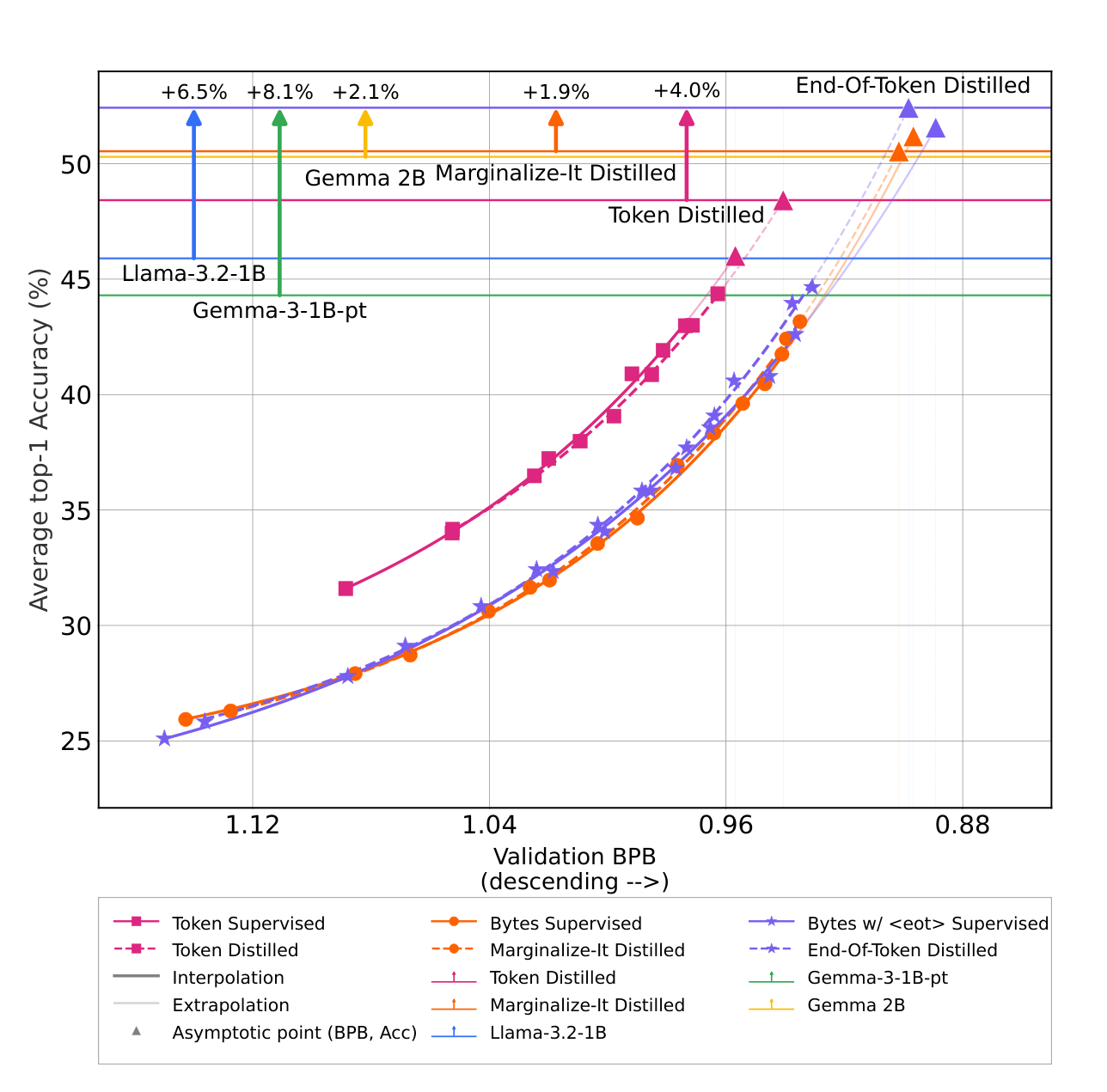
Figure 1 是全文的结论图:横轴是 validation BPB(向右递减),纵轴是六个 benchmark 上的平均 top-1 准确率。实线是插值区间、虚线是外推区间,每条曲线末端的点是该配置的渐近点 $(c, a^\star)$。结论一目了然:End-Of-Token Distilled 的渐近点最高,比 Token Distilled 高 4.0%、比 Marginalize-It Distilled 高 1.9%,并且超过 Llama-3.2-1B / Gemma-3-1B-pt / Gemma 2B 分别 6.5% / 8.1% / 2.1%。
核心方法一:Marginalize-It —— 单次前向的近似 logit 转换¶
问题的形式化¶
教师在每个位置给出一个 $|V|$ 维的 next-token logit 张量($V$ 是 BPE 词表)。同时我们知道 $V$ 中每个 token 解码后的 byte 序列。要把这个 token 分布"摊开"到 byte 位置上,需要对每个 byte 位置 $k$ 求出 $P(b \mid \text{gold}[:k], \text{context})$。
Marginalize-It 的做法¶
- 第一个 byte $B_1$:对整个词表 $V$ 按 token 的首字节做边缘化(把所有首字节相同的 token 概率加起来)。这一步是精确的。
- 后续 byte $B_k$($k \ge 2$):把词表限制到前缀与 ground-truth bytes 相匹配的那些 token,在这个子集上归一化后再按第 $k$ 个字节边缘化。这一步只是近似。
近似在哪里失效¶
论文用一个精心构造的例子说明。考虑 tokenized prompt Tiramisu = [<bos>, T, iram, isu, <eos>],关注 token iram 之后的 next-token 分布(ground truth 是 isu)。
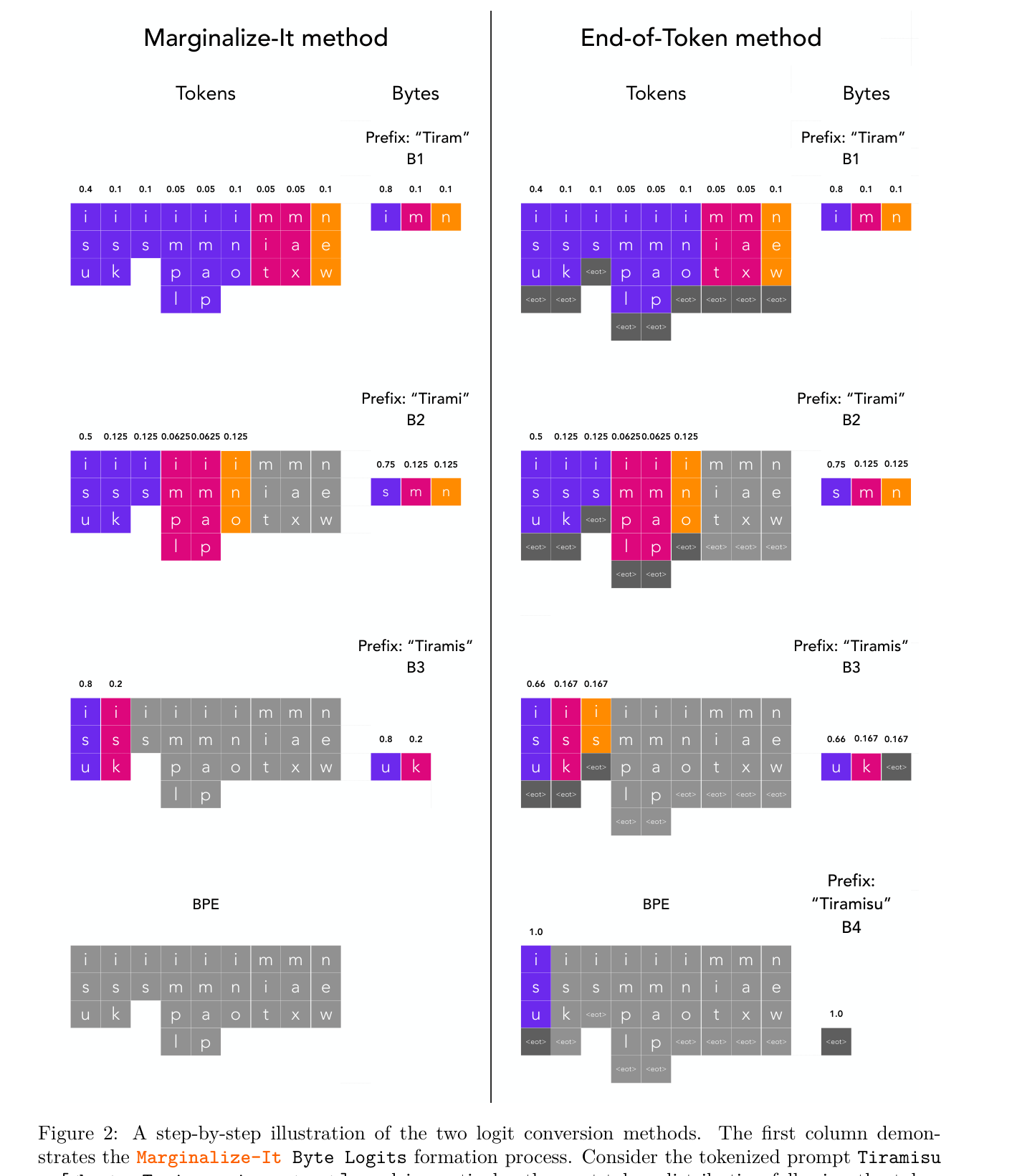
要预测 $B_3$(即 Tiramis 之后的那个字节),Marginalize-It 会把词表限制到"前缀为 is 且字节长度 ≥ 3"的 token,于是只剩下 isu(概率 0.5)和 isk(概率 0.125)。token is 本身(概率 0.125)被静默丢弃了——因为它的字节长度只有 2,不满足"长度 ≥ 3"。剩余概率被重新归一化:
$$P(\texttt{isu}) = \frac{0.5}{0.5 + 0.125} = 0.8, \qquad P(\texttt{isk}) = \frac{0.125}{0.5 + 0.125} = 0.2 \tag{1}$$
要修掉这个问题,理论上只需拿到 token is 的 next-token 分布——但那需要对序列 [<bos>, T, iram, is] 再跑一次教师前向。对长序列而言,为了得到精确转换所需的额外前向次数会迅速变得不可行。这正是 Hayase et al. (2025) 和 Phan et al. (2024) 的方法代价高昂的根源。
训练时使用的 byte 序列是:[<bos>,T,i,r,a,m,i,s,u,<eos>]。Marginalize-It 在全文中作为主基线。
核心方法二:End-Of-Token —— 用 <eot> 把残余质量精确吸收¶
两处改动¶
End-Of-Token 本质上就是 Marginalize-It 加两个改动:
- 构造 byte logit 时,在每个 BPE token 末尾追加一个
<eot>token(Figure 2 第二列); - 把 byte 词表扩大一位来存放
<eot>的概率,然后照常沿 byte 位置做边缘化。
训练时,在预训练数据的每个 BPE token 之后都插入 <eot>:
[<bos>, <eot>, T, <eot>, i, r, a, m, <eot>, i, s, u, <eot>, <eos>, <eot>]。
为什么这样就精确了¶
回到同一个例子。计算 $B_3$ 时,End-Of-Token 会考虑所有前缀为 is 的 token,包括 is 自己——因为加了 <eot> 之后,is<eot> 的字节长度也变成了 3,不再被"长度 ≥ 3"的条件筛掉。前缀为 is 的总概率是 $0.5 + 0.125 + 0.125 = 0.75$:
$$P(\texttt{isu<eot>}) = \frac{0.5}{0.75} = 0.667, \quad P(\texttt{isk<eot>}) = \frac{0.125}{0.75} = 0.167, \quad P(\texttt{is<eot>}) = \frac{0.125}{0.75} = 0.167 \tag{2}$$
is 的所有可能续写的概率质量被吸收进 <eot> 这个 token。这个转换是精确的,且不需要对教师做任何额外前向。
一个意料之外的副作用:多花的算力本身就是收益¶
插入 <eot> 有一个作者称之为"unintended but remarkable"的后果:由于平均每 ≈4.5 个字节就多出一个 <eot>,在固定数据量下 End-Of-Token-1B 要多花 ≈30.94% 的算力(每 token 对应 5.5 个单元而非 4.5 个)。论文后面会证明,这多花的算力本身就进一步抬高了渐近性能——这是一个独立于"分布保真"之外的第二重收益。
伪代码¶
import numpy as np
EOT = 256  # end-of-token symbol (index 256 when use_eot=True)

def byte_probabilities(probs, token_to_bytes, lengths, gold, use_eot=False):
    """Byte distributions P(b | gold[:k], context) for k = 0..len(gold)-1.
    probs (vocab_size):              token probabilities.
    token_to_bytes (vocab_size, max_len): per-token bytes, -1 padded.
    lengths (vocab_size):            true byte length.
    gold:                            byte sequence to condition on.
    use_eot: if True, alphabet is {0..255} U {EOT} (size 257) else 256.
    """
    n_bytes = 257 if use_eot else 256
    live = np.ones(len(probs), dtype=bool)
    dist = []
    for k in range(len(gold)):
        active = live & (lengths > k)
        bytes_at_k = token_to_bytes[:, k]
        accum = np.bincount(bytes_at_k[active], probs[active], minlength=n_bytes)
        total = accum.sum()
        dist.append(accum / total if total > 0 else accum)
        live &= (bytes_at_k == gold[k]) & (lengths > k + 1)
    return dist
注意 live 这一行:它同时施加了「前缀匹配 ground-truth byte」与「长度 > k+1」两个条件。Marginalize-It 的全部误差都来自第二个条件把"恰好在此结束"的 token 漏掉了;<eot> 的作用就是让这类 token 的长度多出 1,从而落回 live 集合里。
四种特殊情形(附录 F.2)¶
论文把 byte logit 转换拆成四种情形逐一分析:
| 情形 | 条件 | Marginalize-It | End-Of-Token |
|---|---|---|---|
| I | 预测 token 的首字节 | 精确(对全词表边缘化) | 精确 |
| II | 中间字节,且词表中所有非零概率的候选 token 与 ground-truth token 长度相同 | 精确 | 精确 |
| III | 中间字节,存在同前缀但字节长度更短的非零概率 token | 有偏:漏掉 [is, ooo]、[is, oo]、[is, uuu] 等分词路径 |
精确(is<eot> 长度变 3,不再被漏) |
| IV | 中间字节,存在同前缀但字节长度更长的非零概率 token | 有偏:基于 ground-truth token is 做条件,漏掉 isu、isk 的贡献 |
精确 |
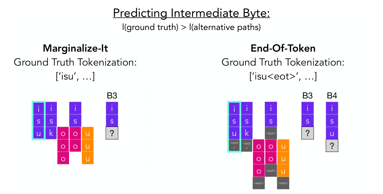
也就是说:只有当 BPE 的字节分解在给定前缀下是"长度齐整"的(情形 I、II),Marginalize-It 才恰好精确。真实 BPE 词表几乎处处不满足这个条件,所以 Marginalize-It 在实际语料上处处有偏。
实验设置¶
六个场景:两轴笛卡尔积¶
研究沿两个轴做受控扫描:tokenization scheme(Tokens / Bytes / Bytes w/ <eot>)× 训练目标(Cross-Entropy 监督 / Distillation)。
| Experiment | Tokenization | Vocab. size | Objective | Architecture | Model size | FLOPs/unit |
|---|---|---|---|---|---|---|
| Token Supervised | Tokens (Llama 3-8B) | 128,256 | Cross-Entropy | Token-1B | 1.81B | $8.18\times10^9$ |
| Token Distilled | Tokens (Llama 3-8B) | 128,256 | Distillation (top-k) | Token-1B | 1.81B | $8.18\times10^9$ |
| Bytes Supervised | Bytes (256 + 4 special) | 260 | Cross-Entropy | Bytes-1B | 1.28B | $8.81\times10^9$ |
| Marginalize-It Distilled | Bytes (256 + 4 special) | 260 | Distillation (approximate) | Bytes-1B | 1.28B | $8.81\times10^9$ |
Bytes w/ <eot> Supervised |
Bytes w/ <eot> (256 + 5 special) |
261 | Cross-Entropy | End-Of-Token-1B | 1.28B | $9.44\times10^9$ |
| End-Of-Token Distilled | Bytes w/ <eot> (256 + 5 special) |
261 | Distillation (Exact) | End-Of-Token-1B | 1.28B | $9.44\times10^9$ |
(Table 1)
模型架构与 FLOP 计算(Table 9)¶
三个架构的层参数完全相等(1,284,608,000),差异只来自词表大小(embedding / de-embedding)与序列长度:
| Property | Formula | Token-1B | Bytes-1B | End-Of-Token-1B |
|---|---|---|---|---|
| Model Dimension $d$ | — | 2048 | 2048 | 2048 |
| FFN dimension $d_{ffn}$ | $\lceil 4\cdot\frac{2}{3}\cdot\frac{d}{256}\rceil\cdot 256$ | 5632 | 5632 | 5632 |
| Number of Layers $n$ | — | 25 | 25 | 25 |
| Number of Heads | — | 16 | 16 | 16 |
| Vocabulary size $V$ | — | 128,256 | 260 | 261 |
| Attention Params / Layer | $4d^2$ | 16,777,216 | 16,777,216 | 16,777,216 |
| FFN Params / Layer | $3\cdot d\cdot d_{ffn}$ | 34,603,008 | 34,603,008 | 34,603,008 |
| RMSNorm Params / Layer | $2d$ | 4,096 | 4,096 | 4,096 |
| Total Layer Parameters | $n(N_{attn}+N_{ffn}+N_{norm})$ | 1,284,608,000 | 1,284,608,000 | 1,284,608,000 |
| Total Non-Embedding Params | $N_{layers}+N_{preoutputnorm}+d\cdot V$ | 1,547,278,336 | 1,285,142,528 | 1,285,144,576 |
| Total Parameters | $N_{nonembed}+d\cdot V$ | 1,809,946,624 | 1,285,675,008 | 1,285,679,104 |
| Sequence Length $l$ | — | 2048 | 9216 | 11264 |
| Self Attention FLOPs | $4n\cdot(d/n_{heads})\cdot n_{heads}\cdot\frac{l+1}{2}$ | 209,817,600 | 943,820,800 | 1,153,536,000 |
| QKVO FLOPs | $(2+2)\cdot 2\cdot n\cdot d^2$ | 838,860,800 | 838,860,800 | 838,860,800 |
| Feed Forward FLOPs | $2\cdot n\cdot 2\cdot d\cdot d_{ffn}$ | 1,153,433,600 | 1,153,433,600 | 1,153,433,600 |
| De-Embedding FLOPs | $2\cdot d\cdot|V|$ | 525,336,576 | 1,064,960 | 1,069,056 |
| Total FLOPs per unit | $3(F_{attn}+F_{qkvo}+F_{ffn}+F_{deemb})$ | 8,182,345,728 | 8,811,540,480 | 9,440,698,368 |
这张表值得停下来看:Token-1B 虽然"层参数相同",但总参数是 1.81B,比两个 byte 模型(1.28B)多了 40%,多出来的全在 embedding/de-embedding 上。反过来,byte 模型为了在固定 context 下装下同样内容,序列长度从 2048 拉到 9216 / 11264,attention FLOPs 因此涨了 4.5×/5.5×。这个非对称性是全文所有结论的物理根源:byte 模型用更少的参数、更多的每字节算力,换来了更低的渐近 BPB。
激活函数用 SwiGLU(Shazeer 2020),整体沿用 Llama-3(Grattafiori et al. 2024)的设计选择。
损失函数¶
标准的知识蒸馏由两项组成,用混合系数 $\alpha$ 控制:$\alpha = 0$ 退化为纯监督(cross-entropy),$\alpha = 1$ 为纯蒸馏。
$$\mathcal{L}_{KD} = \alpha \cdot \mathcal{L}_{KL} + (1-\alpha)\cdot \mathcal{L}_{CE} \tag{3}$$
$$\mathcal{L}_{KL} = \frac{1}{n}\sum_{t=1}^{n}\sum_{c} p_T(c \mid x_{<t}) \log \frac{p_T(c \mid x_{<t})}{p_S(c \mid x_{<t})} \tag{4}$$
$$\mathcal{L}_{CE} = -\frac{1}{n}\sum_{t=1}^{n}\sum_{c} y_{t,c} \log p_S(c \mid x_{<t}) \tag{5}$$
其中 $t$ 是序列位置索引,$n$ 是序列长度,$c$ 遍历词表 $V$,$y_{t,c}\in\{0,1\}$ 是 ground-truth 的 one-hot 指示,$p_T$ / $p_S$ 分别是教师 / 学生的预测分布。
训练细节¶
- 教师:Llama3-8B(Grattafiori et al. 2024)。其在验证集上的 BPB 为 0.85511——这是全部曲线的"地板"。
- 数据:Llama-2(Touvron et al. 2023)的预训练混合。两套 tokenizer:BPE-Tiktoken(Llama3-8B)与 byte tokenizer(256 UTF-8 字节 + 4 个特殊 token)。
- 优化器:AdamW,$\beta_1=0.9$、$\beta_2=0.95$,cosine LR schedule,warmup = 各数据规模最大步数的 10%,independent weight decay $10^{-4}$(Kosson et al. 2025),grad clip norm 1.0。
- 三个 peak learning rate:$\{1\text{e-}3,\ 4\text{e-}3,\ 8\text{e-}3\}$。正文分析用 4e-3,附录给出全部三个。
- 序列长度与 batch:Token-1B 用 2048。byte transformer 最初按"完全相同的 context 与数据"($8\text{K}\times4\times64 = 2\text{M}$ bytes / step)训练时出现 loss spike;为了稳住,作者启用 qk-norm 并把序列长度设为 Bytes-1B 9216、End-Of-Token-1B 11264,同时保持 ≈0.5M 单元的 global batch size。若 2048 个 token 对应的字节序列超长就截断,短则 pad。每个 run 用 64 张 H200。
- 作者明确指出一个重要后果:在相同算力预算下,byte 模型实际见到的数据量远少于 token 模型。
- 数据规模:Tokens 15B–500B;Bytes 16B–968B;Bytes w/
<eot>20B–1.2T。
BPB 的定义¶
跨 tokenizer 公平比较必须放弃 token 级 loss,用 bits-per-byte:把验证集上的总 cross-entropy 除以总字节数 $B$ 并换算成 bit。
$$\mathrm{BPB} = \frac{\mathcal{L}_{CE}(x)\cdot \log_2 e}{B} \tag{6}$$
直观上它衡量"模型平均用多少 bit 表示一个字节的数据"。
存储成本的对齐(Table 10)¶
为了让对比公平,作者让同等数据量下 token logit 与 byte logit 占用相同存储,反解出 top-k 的 k:
| Token type | Data Attribute | Datatype | Bytes/value | # Values | Total Cost |
|---|---|---|---|---|---|
| BPE-tiktoken | Token Logit values | float32 | 4 | $k$ | $4k + 4k + 4$ |
| Token Logit indices | int32 | 4 | $k$ | ||
| Tokens | int32 | 4 | 1 | ||
| Bytes | Byte Logits | float32 | 4 | $260\times4.5$ | $4680 + 9$ |
| Bytes | int16 | 2 | 4.5 |
令两者相等解得 $k = 4685/8 = 585.625 \approx 600$。因此受控对比中,每个 BPE token 存 600 个 logit,而 byte 侧存全部 260 个值。注意 BPE 侧用的是稀疏表示(值 + 索引),byte 侧存的是完整分布。
评测基准¶
三大类共 8 个 benchmark:
- Multiple Choice QA:ARC-Easy、ARC-Challenge(P. Clark et al. 2018)、HellaSwag(Zellers et al. 2019)、PIQA(Bisk et al. 2020)
- Language Generation:MBPP(Austin et al. 2021,Pass@1)、Natural Questions(Kwiatkowski et al. 2019,Exact Match)
- Machine Translation:Flores(Goyal et al. 2022)英→德、德→英,BLEU(Papineni et al. 2002)
开源模型用 lm-evaluation-harness(Gao et al. 2024)评测。
Scaling Trend I:Validation BPB vs Training FLOPs¶
幂律形式¶
对每个场景拟合:
$$y = b \cdot x^a + c \tag{7}$$
$x$ 是训练 FLOPs,$y$ 是该算力预算下的 BPB,$c$ 是渐近(不可约)BPB。
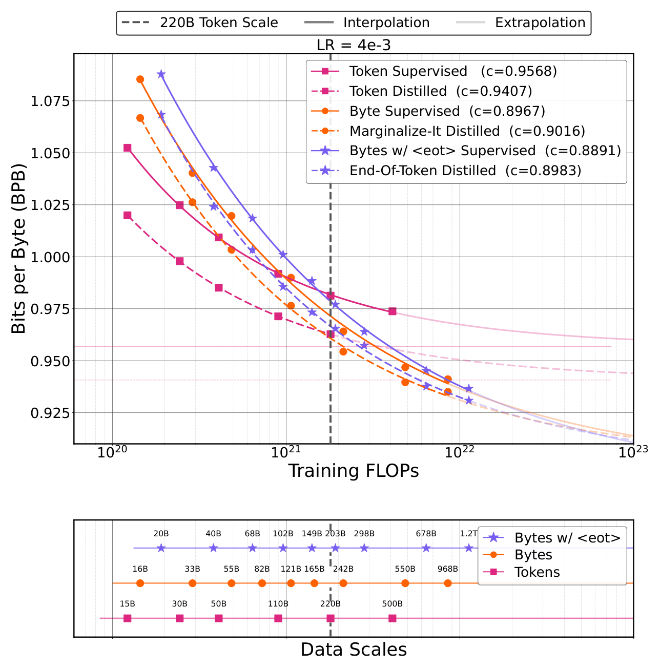
拟合结果(LR = 4e-3,Table 2 + Table 13)¶
| Scenario | Equation | $R^2$ |
|---|---|---|
| Token Supervised | $y = 1.075\times10^{9}\cdot x^{-0.500369} + 0.9568$ | 0.9999 |
| Token Distilled | $y = 2.803\times10^{8}\cdot x^{-0.475375} + 0.9407$ | 1.0000 |
| Bytes Supervised | $y = 4.467\times10^{6}\cdot x^{-0.365844} + 0.8967$ | 0.9980 |
| Marginalize-It Distilled | $y = 2.706\times10^{7}\cdot x^{-0.407427} + 0.9016$ | 0.9974 |
Bytes w/ <eot> Supervised |
$y = 3.080\times10^{6}\cdot x^{-0.354594} + 0.8891$ | 0.9982 |
| End-Of-Token Distilled | $y = 2.734\times10^{7}\cdot x^{-0.404740} + 0.8983$ | 0.9990 |
三个学习率的完整幂律(Table 11)与渐近 BPB(Table 12):
| Method | $c$ (LR=1e-3) | $c$ (LR=4e-3) | $c$ (LR=8e-3) |
|---|---|---|---|
| Token Supervised | 0.9559 | 0.9568 | 0.9575 |
| Token Distilled | 0.9452 | 0.9407 | 0.9441 |
| Bytes Supervised | 0.9124 | 0.8967 | 0.9080 |
| Marginalize-It Distilled | 0.9092 | 0.9016 | 0.9133 |
Bytes w/ <eot> Supervised |
0.9074 | 0.8891 | 0.9165 |
| End-Of-Token Distilled | 0.9074 | 0.8983 | 0.9073 |
算力/单位数据 与渐近 BPB 的单调关系(Table 3)¶
这张表是全文最关键的机制性证据之一。"一个单位"对 token 模型是 1 个 BPE token,对 byte 模型是 1 个 byte(平均 4.5 个 byte = 1 个 token;加 <eot> 后是 5.5 个单元):
| Method | Architecture | FLOPs / Unit | Units per Token | Total FLOPs per Token | Asymptotic BPB (4e-3) |
|---|---|---|---|---|---|
| Token Supervised | Token-1B | $8.18\times10^9$ | 1.0 | $8.18\times10^9$ | 0.9568 |
| Bytes Supervised | Bytes-1B | $8.81\times10^9$ | 4.5 | $39.65\times10^9$ | 0.8967 |
Bytes w/ <eot> Supervised |
End-Of-Token-1B | $9.44\times10^9$ | 5.5 | $51.92\times10^9$ | 0.8891 |
| Token Distilled | Token-1B | $8.18\times10^9$ | 1.0 | $8.18\times10^9$ | 0.9407 |
| Marginalize-It Distilled | Bytes-1B | $8.81\times10^9$ | 4.5 | $39.65\times10^9$ | 0.9016 |
| End-Of-Token Distilled | End-Of-Token-1B | $9.44\times10^9$ | 5.5 | $51.92\times10^9$ | 0.8983 |
在固定数据量上花的算力越多,渐近 BPB 越低——这在监督和蒸馏两组里都单调成立。End-Of-Token-1B 相比 Bytes-1B 多花 ≈30.94% 的每 token 算力($51.92/39.65 = 1.3094$),这就是那多出来的 <eot> 的代价,也是它的收益来源。
五条观察¶
Marginalize-It Distilled(近似)和End-Of-Token Distilled(精确)都优于各自的监督对照。- Marginalize-It 尽管是近似,实践中工作得很好;End-Of-Token 是精确的,相对监督训练给出一致的提升。
- Token-1B 在低算力预算下 BPB 最低,但饱和最快;End-Of-Token-1B 起点最差却给出无限算力下最好的渐近值;Bytes-1B 在起点和终点都被夹在中间。
- 渐近上,监督与蒸馏两组都满足:End-Of-Token-1B BPB < Bytes-1B BPB < Token-1B BPB。同一 tokenization 下,监督与蒸馏的渐近值差异很小。
- 在 ≈$1.8\times10^{21}$ FLOPs 附近,
Token Supervised的 BPB 是六条曲线里最高的——其他五条都更低。这是否意味着那五个模型在该预算下都更好?第 5 节给出的答案是:不是。
Scaling Trend II:下游任务性能 vs Training FLOPs¶
Multiple Choice QA(Figure 4)¶
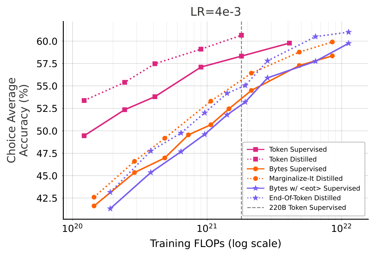
- 六个场景的平均选择题准确率都随算力提升,且蒸馏模型一致优于监督模型(逐 benchmark 也成立)。
- Token-1B 起步最好,在低算力预算下超过所有 byte 曲线;byte 曲线起步更差但改善速度更快,最终追上。
- 在四个 byte 实验内部比较:
End-Of-Token-1B(监督与蒸馏)都起步更差,但最终反超对应的 Bytes-1B。 - Token-1B(监督与蒸馏)开头最好但明显在饱和——与 BPB 曲线的形态一致。
- 在 220B token 监督预算这个点上,只有蒸馏 Token-1B 超过了它的监督对照;四条 byte 曲线(监督与蒸馏)都明显更差——这与第 4 节的观察 5 直接矛盾。
Language Generation(Figure 5)¶
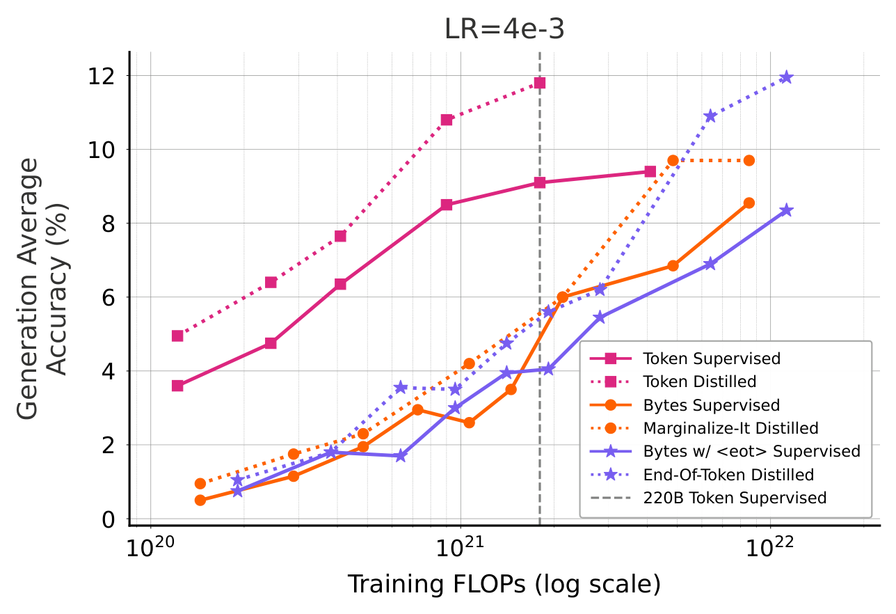
趋势与选择题相似,但 Token-1B 的饱和效应没那么明显,作者推测是因为这类任务本身难得多(MBPP Pass@1 与 NQ Exact Match 的绝对值都只有个位数到十几)。同样地,在 $1.8\times10^{21}$ FLOPs 预算下只有 Token Distilled 表现更好,其余四条 byte 曲线在多数情况下都差很多。
Machine Translation(Figure 6)¶
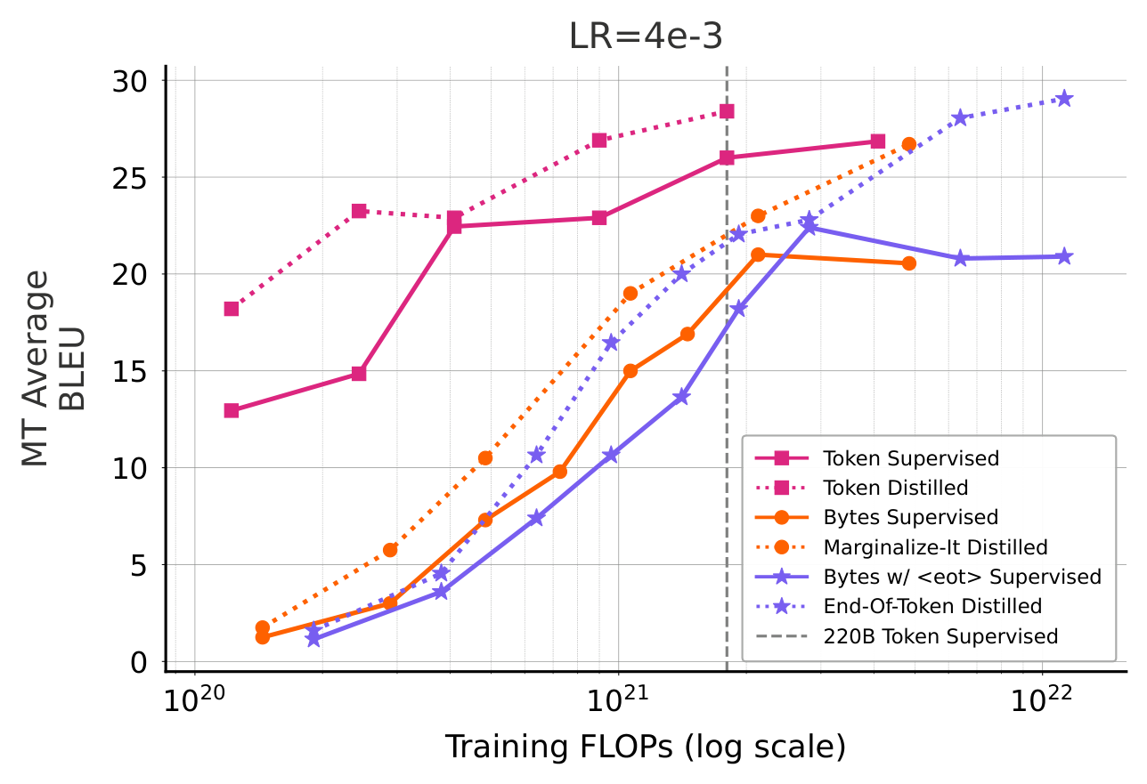
- byte 模型的 BLEU 呈明显的 S 形:低算力区几乎不动,中段陡升,高算力区饱和。
- 这里同样反驳了第 4 节的观察 5。
End-Of-Token Distilled因为精确保留教师分布,相对Bytes w/ <eot> Supervised提升显著。
小结:BPB 更低 ≠ 模型更好¶
对我们观察到的数据点,蒸馏模型确实比其监督对照同时拥有更低的 BPB 和更好的整体下游表现。但这条规律在 Token-1B 与 Bytes-1B / End-Of-Token-1B 之间不成立:Token-1B 可以 BPB 更差却下游更好——220B token 数据规模处就是如此。
Scaling Trend III:下游误差 vs Validation BPB¶
三类任务上的观察¶
沿用 Gadre et al. (2024) 的 downstream scaling law 形式,把 Average top-1 error(即 $1 - \%\text{Accuracy}$) 对 validation BPB 作图。
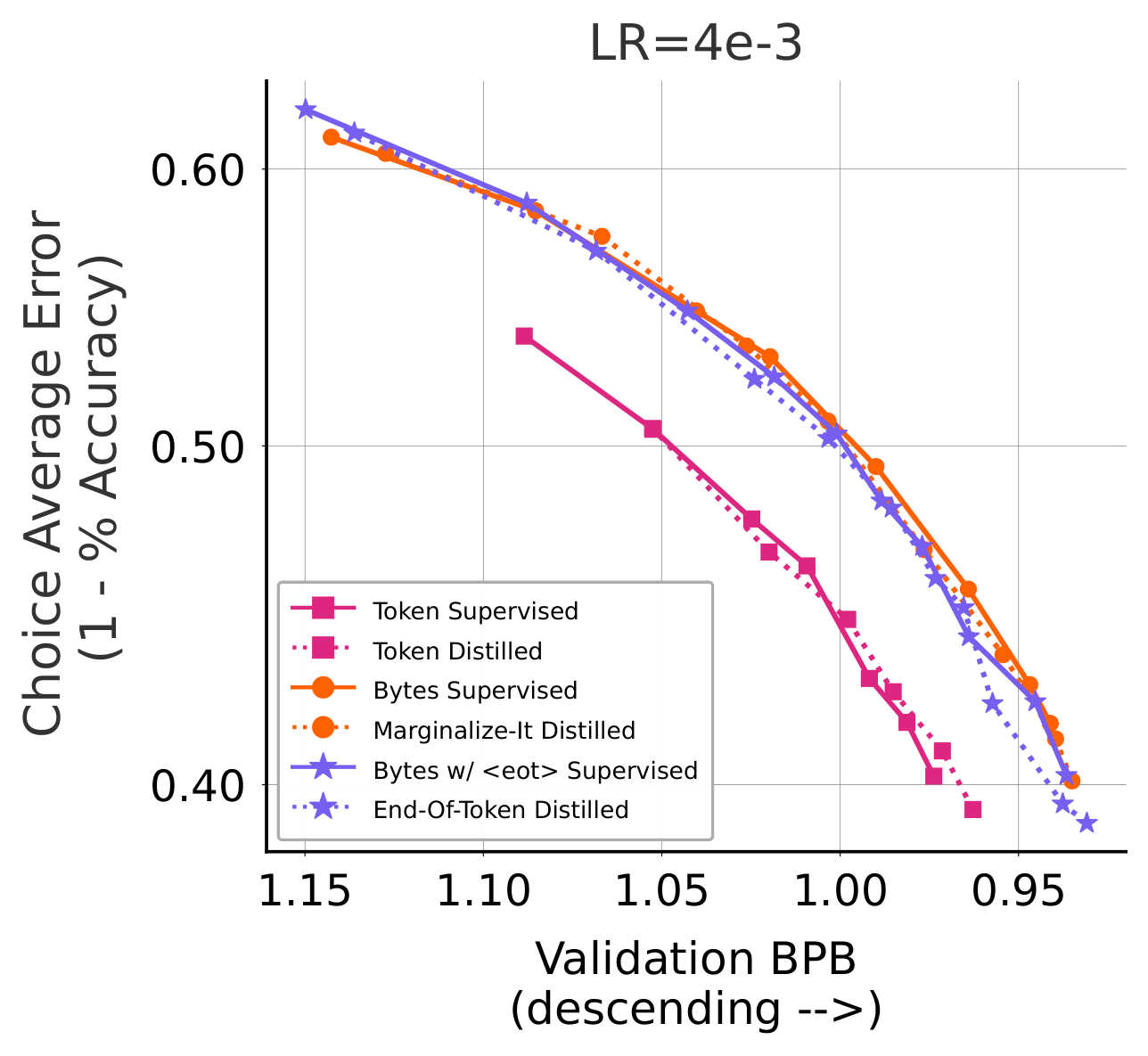
选择题上的三条观察:
- 六条曲线形态显著不同。在相同 BPB 下它们对应的错误率相差悬殊;iso-error 线与 End-Of-Token 曲线、Token 曲线的交点落在完全不同的算力预算上。
- 改变 tokenization(也就是改变"为固定数据量花多少算力")能戏剧性地改变标度行为。
- 训练目标(监督 vs 蒸馏)同样改变标度行为。
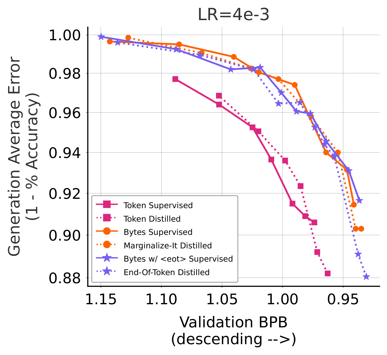
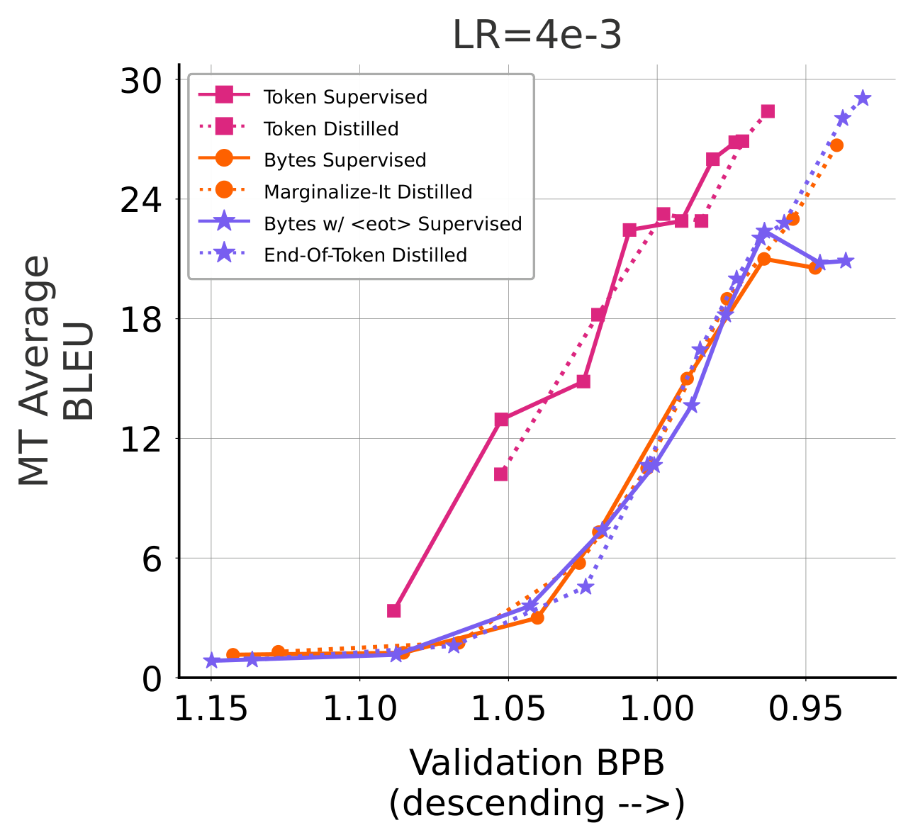
语言生成任务上同样是"相同 BPB 对应不同下游表现"。机器翻译上,三类 tokenization 的标度行为互不相同,而 End-Of-Token 蒸馏相比噪声很大的 Bytes w/ <eot> Supervised 曲线呈现单调趋势——这一点后面在讨论里会被作为"蒸馏让标度曲线更可预测"的证据。
拟合下游误差标度律¶
$$z(y) = \epsilon - k\cdot e^{-\gamma y} \tag{8}$$
$y$ 是 validation BPB,$z(y)$ 是四个选择题 + 两个生成任务共 6 个 benchmark 上的平均 top-1 错误率,$\epsilon, k, \gamma$ 由数据拟合。曲线的右端被 Table 2 给出的渐近 BPB $c$ 截断。
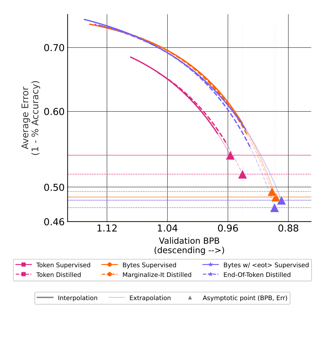
LR = 4e-3 的拟合式(Table 4):
| Method | Model | Scaling law $z(y)$ |
|---|---|---|
| Token Supervised | Token-1B | $0.7501 - 934.3212\, e^{-8.7782y}$ |
| Token Distilled | Token-1B | $0.7383 - 1292.0124\, e^{-9.2132y}$ |
| Bytes Supervised | Bytes-1B | $0.7686 - 1231.1241\, e^{-9.3532y}$ |
| Marginalize-It Distilled | Bytes-1B | $0.7721 - 1137.3004\, e^{-9.2265y}$ |
Bytes w/ <eot> Supervised |
End-Of-Token-1B | $0.7972 - 185.6303\, e^{-7.1822y}$ |
| End-Of-Token Distilled | End-Of-Token-1B | $0.7776 - 827.6076\, e^{-8.8125y}$ |
渐近性能上界¶
把渐近 BPB $c$ 代回式 (8) 得渐近误差 $z^\star$,渐近准确率 $a^\star = 1 - z^\star$:
$$z^\star = \epsilon - k\cdot e^{-\gamma c}, \qquad a^\star = 1 - z^\star \tag{9}$$
三个学习率的完整结果(Table 5 / Table 15):
| Method | $c$ (1e-3) | $a^\star$ (1e-3) | $c$ (4e-3) | $a^\star$ (4e-3) | $c$ (8e-3) | $a^\star$ (8e-3) |
|---|---|---|---|---|---|---|
| Token Supervised | 0.9559 | 44.2 | 0.9568 | 46.0 | 0.9575 | 45.8 |
| Token Distilled | 0.9452 | 46.6 | 0.9407 | 48.4 | 0.9441 | 45.7 |
| Bytes Supervised | 0.9124 | 48.7 | 0.8967 | 51.2 | 0.9080 | 47.9 |
| Marginalize-It Distilled | 0.9092 | 49.0 | 0.9016 | 50.5 | 0.9133 | 47.0 |
Bytes w/ <eot> Supervised |
0.9074 | 48.5 | 0.8891 | 51.6 | 0.9165 | 46.8 |
| End-Of-Token Distilled | 0.9074 | 49.7 | 0.8983 | 52.4 | 0.9073 | 49.8 |
五条结论:
- 蒸馏 Token-1B 渐近上优于监督对照。
End-Of-Token Distilled渐近上同时优于Token Distilled和Bytes w/ <eot> Supervised。- 蒸馏 Bytes-1B(Marginalize-It)与其监督对照持平甚至更差(51.2 → 50.5),作者归因于它用的是教师分布的近似。但它仍然超过渐近的蒸馏 Token-1B。这是"近似转换会损失收益"的直接证据。
- 多花 ≈30.94% 的算力换来
Bytes w/ <eot> Supervised优于Bytes Supervised的渐近行为。 End-Of-Token Distilled的渐近下游表现优于Bytes w/ <eot> Supervised。
注意 End-Of-Token Distilled 是唯一一个在三个学习率下都排第一的配置(49.7 / 52.4 / 49.8),而其他配置在 8e-3 下大幅退化(例如 Bytes w/ <eot> Supervised 从 51.6 掉到 46.8)。这条鲁棒性证据在正文中没有被强调,但它比单点 +4% 更有说服力。
为什么 BPB 不能跨 tokenization / 目标比较¶
作者的解释是:这些差异源于"在少量数据上每单位花大量算力" vs "在大量数据上每单位花少量算力"这两种配置在固定总算力下学到的概率分布本身不同。虽然所有 Bytes-1B 和 End-Of-Token-1B 都超过了 Token Supervised 的 BPB 曲线,它们在各个 benchmark 上的下游表现却更差——这证伪了第 4 节的观察 5,并强调了"上线前必须做这一步最终校准"。
何时该选 byte 蒸馏:Feather Plot 与交叉点¶
Feather Plot¶
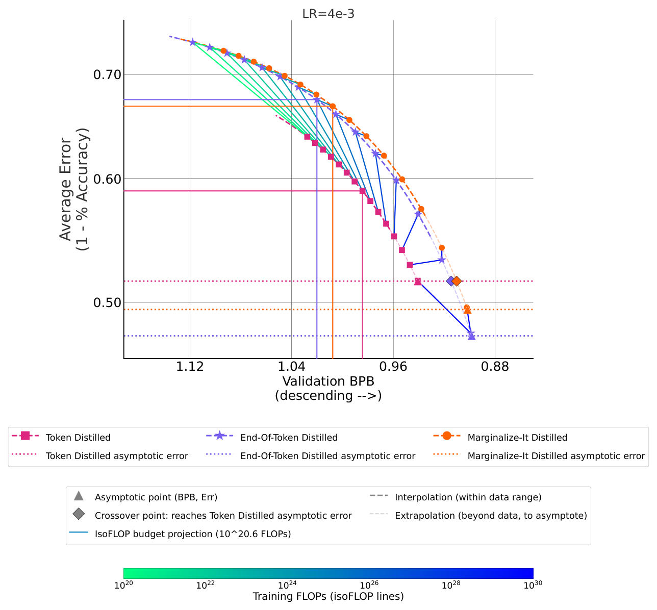
Feather Plot 是本文自造的一种可视化:在 downstream-error vs validation-BPB 平面上,把等 FLOPs 的点用线连起来(形如羽毛的横纹)。构造方式是:从 FLOP 区间 $[f_1, f_2]$ 采样 $x$ → 用式 (7) 算出 BPB $y$ → 用式 (8) 算出下游误差 $z(y)$ → 把三条蒸馏曲线(Token / Marginalize-It / End-Of-Token)上的同 FLOPs 点连线。
它回答的问题是:在给定算力预算下,此刻哪条路线领先? 三条观察:
- 低算力预算下,蒸馏 Token-1B 显著领先;
- 随着预算增长,蒸馏 End-Of-Token-1B 先反超 Bytes-1B;
- 最终 End-Of-Token-1B 追上并持续改善到它的渐近值。
图里特意标了 $10^{20.63}$ FLOPs 这个随机采样点:在那个预算下 Token 蒸馏领先很多,两条 byte 路线都落后——"什么时候该切换"这件事本身强依赖预算。
交叉点计算(Table 6 / Table 16)¶
方法:取 Token Distilled 的渐近 BPB(其幂律的 $c$ 项)→ 过它自己的 benchmark 标度律得到渐近准确率 → 对每个 byte 方法反解它自己的标度律,求出要达到该准确率所需的 BPB → 再反解它自己的 BPB–FLOPs 幂律,得到所需训练算力。
| LR | Method | Token Dist. BPB | Accuracy | Method BPB | Method Training FLOPs |
|---|---|---|---|---|---|
| 1e-3 | Marginalize-It Distilled | 0.9452 | 46.6% | 0.9195 | $7.05\times10^{22}$ |
| 1e-3 | End-Of-Token Distilled | 0.9452 | 46.6% | 0.9216 | $3.91\times10^{22}$ |
| 4e-3 | Marginalize-It Distilled | 0.9407 | 48.4% | 0.9102 | $\mathbf{2.04\times10^{23}}$ |
| 4e-3 | End-Of-Token Distilled | 0.9407 | 48.4% | 0.9145 | $\mathbf{6.33\times10^{22}}$ |
| 8e-3 | Marginalize-It Distilled | 0.9441 | 45.7% | 0.9197 | $9.27\times10^{22}$ |
| 8e-3 | End-Of-Token Distilled | 0.9441 | 45.7% | 0.9256 | $2.13\times10^{22}$ |
End-Of-Token 达到 Token 蒸馏渐近性能所需的算力,比 Marginalize-It 少 3.2×–4.4×(4e-3 下 $6.33\times10^{22}$ vs $2.04\times10^{23}$)。
数据与存储效率(Table 7 / Table 17)¶
| Metric | Formula | Marginalize-It Distilled | End-Of-Token Distilled |
|---|---|---|---|
| Training FLOPs | 达到 Token 蒸馏渐近性能所需算力 | $2.04\times10^{23}$ | $6.33\times10^{22}$ |
| $\mathrm{FPU}_{bytes}$ | 每 byte 单元的 FLOPs | $8.81\times10^{9}$ | $9.44\times10^{9}$ |
| $\mathrm{FPU}_{tokens}$ | 每 token 的 FLOPs | $8.18\times10^{9}$ | $8.18\times10^{9}$ |
| Byte Units | FLOPs / $\mathrm{FPU}_{bytes}$ | $2.32\times10^{13}$ | $6.70\times10^{12}$ |
| Multiplier | 实际内容占比 | 1 | 4.5/5.5 |
| Bytes | Byte Units × Multiplier | $2.32\times10^{13}$ | $5.48\times10^{12}$ |
| Tokens | FLOPs / $\mathrm{FPU}_{tokens}$ | $2.50\times10^{13}$ | $7.73\times10^{12}$ |
| Token to Byte | Tokens × 4.5 | $1.12\times10^{14}$ | $3.48\times10^{13}$ |
| Data Savings | Token to Byte / Bytes | 4.85× | 6.35× |
| Storage Savings | Tokens × 4.5 / Byte Units | 4.85× | 5.19× |
Multiplier 那一行是关键细节:End-Of-Token 的序列里每 4.5 个内容字节就夹一个 <eot>,所以 $6.70\times10^{12}$ 个 byte 单元只对应 $5.48\times10^{12}$ 字节的真实文本。扣掉这一项后,End-Of-Token 仍然只需要约六分之一的独特文本(6.35×),并把教师 logit 存储成本降到约五分之一(5.19×)。这两个数在三个学习率下完全一致(4.85×/4.85× 与 6.35×/5.19×),因为它们只取决于架构常数,与拟合出的交叉点无关。
结论:End-Of-Token-1B 的渐近下游表现优于蒸馏 Token-1B,同时只需六分之一的文本数据、五分之一的存储成本,尽管它的总参数量更少(1.28B vs 1.81B)。
与开源权重模型的对比¶
渐近预测 vs 开源模型(Table 8)¶
| Model | Method | Asymptotic Avg. Accuracy (%) |
|---|---|---|
| Token-1B | Token Supervised | 46.0 |
| Token-1B | Token Distilled | 48.4 |
| Bytes-1B | Bytes Supervised | 51.2 |
| Bytes-1B | Marginalize-It Distilled | 50.5 |
| End-Of-Token-1B | Bytes w/ <eot> Supervised |
51.6 |
| End-Of-Token-1B | End-Of-Token Distilled | 52.4 |
| Llama-3.2-1B | Meta AI (2024) | 45.9(≈9T BPE tokens) |
| Gemma-3-1B-pt | Kamath et al. (2025) | 44.3(≈2T BPE tokens) |
| Gemma 2b | Team et al. (2024) | 50.3(≈3T BPE tokens) |
实测 checkpoint(Table 18,LR=4e-3,各自最大数据规模)¶
这张表是全文唯一的实测数字,也是解读全文时最应该对照的一张:
| Model | Data Scale | HellaSwag | PIQA | ARC-Easy | ARC-Challenge | MBPP | NQ | Avg. |
|---|---|---|---|---|---|---|---|---|
| Llama-3.2-1B | 9T | 64.3 | 75.3 | 66.1 | 36.6 | 27.0 | 5.7 | 45.9 |
| Gemma-3-1B-pt | 2T | 62.1 | 74.7 | 72.2 | 38.4 | 9.0 | 9.5 | 44.3 |
| Gemma 2b | 3T | 71.44 | 78.07 | 72.18 | 41.89 | 28.0 | 10.53 | 50.3 |
| Token Supervised | 500B | 63.4 | 74.5 | 65.1 | 36.1 | 8.6 | 10.2 | 43.0 |
| Token Distilled | 220B | 64.2 | 75.7 | 66.4 | 36.3 | 10.6 | 13.0 | 44.4 |
| Bytes Supervised | 880B | 63.9 | 73.1 | 62.6 | 33.8 | 7.0 | 10.1 | 41.8 |
| Marginalize-It Distilled | 880B | 64.9 | 74.5 | 63.6 | 36.6 | 9.4 | 10.0 | 43.2 |
Bytes w/ <eot> Supervised |
880B | 65.6 | 72.0 | 66.3 | 35.1 | 5.6 | 11.1 | 42.6 |
| End-Of-Token Distilled | 880B | 67.1 | 71.7 | 68.3 | 36.9 | 11.2 | 12.7 | 44.6 |
几点必须说清楚:
- 实测层面,
End-Of-Token Distilled(44.6)相对Token Distilled(44.4)只领先 0.2 个点,远不是渐近预测的 +4.0。逐 benchmark 看是有涨有跌:HellaSwag +2.9、ARC-Easy +1.9、MBPP +0.6、ARC-C +0.6,但 PIQA −4.0、NQ −0.3。 - 两者都还没超过 Gemma 2b 的 50.3;所有"超过开源模型"的说法全部是渐近外推。
End-Of-Token Distilled在 MBPP 上 11.2 已经优于 Gemma-3-1B-pt 的 9.0,NQ 上 12.7 优于三个开源模型中的任何一个;但在 HellaSwag/PIQA 这类常识题上仍明显落后 Gemma 2b。Token Distilled只训到 220B token(其他都在 500B–880B),这是因为 token 侧的 logit 存储成本更高——这本身就是论文论点的一个侧面证据,但同时也让"同预算下谁更好"的实测比较不完全对等。
标度律的敏感性分析(附录 D)¶
作者对拟合的稳健性做了三组检查,这部分是本文严谨度的主要来源。
Leave-One-Out(Figure 21)¶
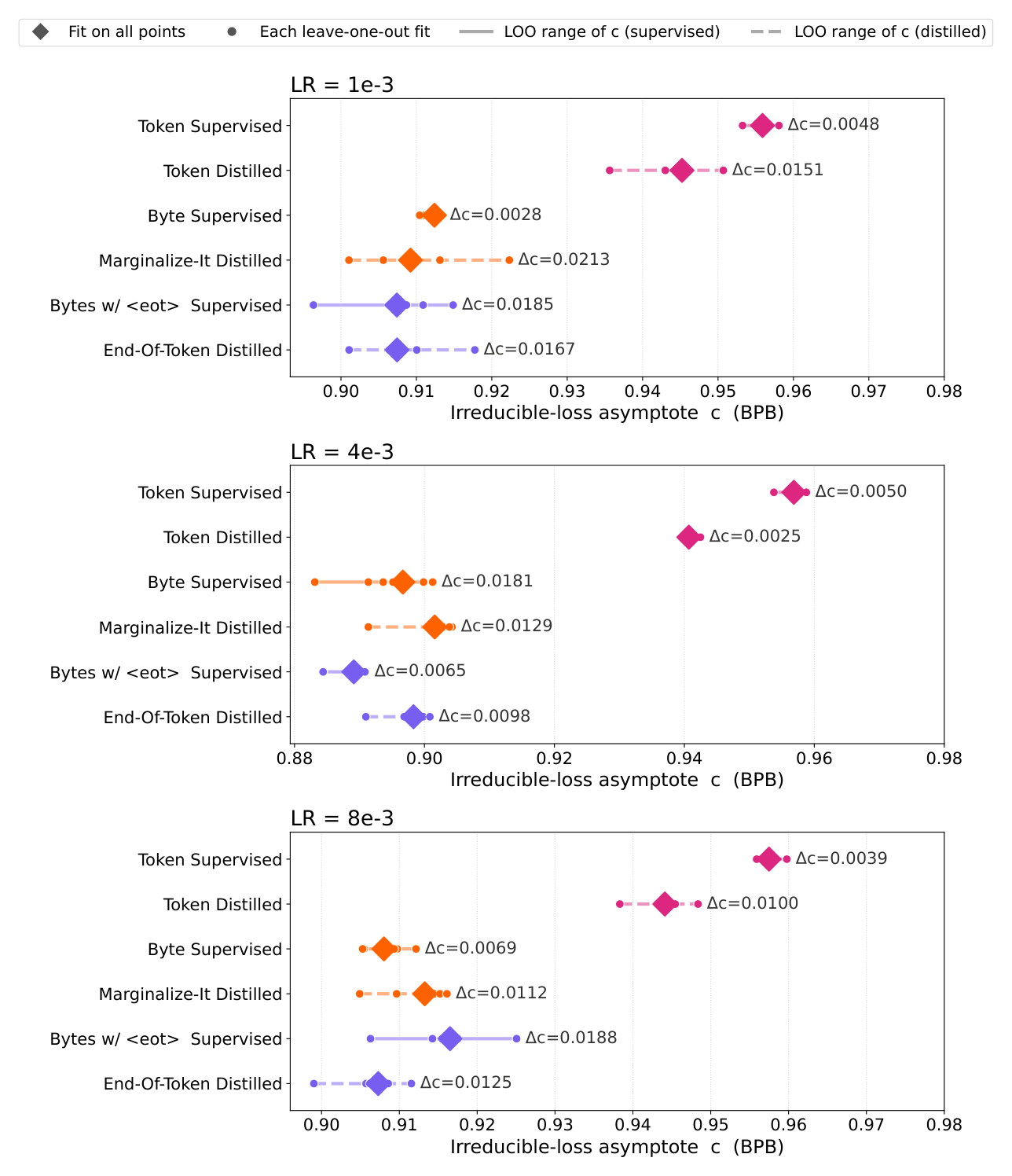
每次丢掉一个数据点重新拟合,看渐近项 $c$ 的散布范围:
| LR | Token Sup. | Token Dist. | Byte Sup. | Marg-It Dist. | Bytes <eot> Sup. |
EoT Dist. |
|---|---|---|---|---|---|---|
| 1e-3 | 0.0048 | 0.0151 | 0.0028 | 0.0213 | 0.0185 | 0.0167 |
| 4e-3 | 0.0050 | 0.0025 | 0.0181 | 0.0129 | 0.0065 | 0.0098 |
| 8e-3 | 0.0039 | 0.0100 | 0.0069 | 0.0112 | 0.0188 | 0.0125 |
结论是 token 曲线的散布普遍小于 byte 与 bytes-w/-<eot> 方法。这一点需要与主结论并读:4e-3 下 End-Of-Token Distilled 的 $c$ LOO 散布是 0.0098,而它与 Token Distilled 的 BPB 差距是 $0.9407 - 0.8983 = 0.0424$——BPB 渐近差距比不确定度大 4 倍多,这一层是稳的。但 BPB→准确率的那一步映射(式 8)没有做同样的 LOO 分析。
残差加权方案(Figure 22)¶
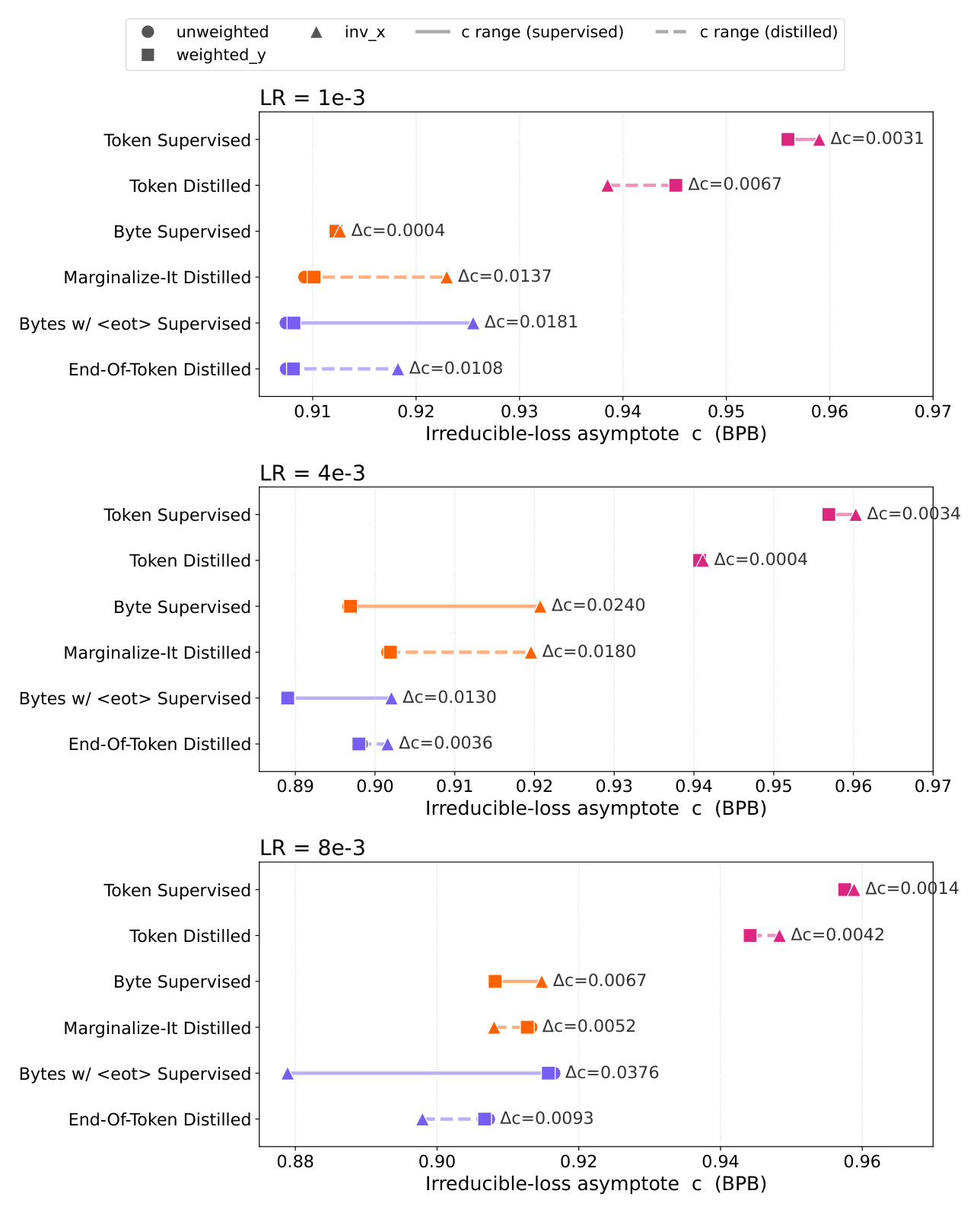
三种 $\sigma$ 选择:unweighted(普通最小二乘)、weighted-y(最小化相对误差 $(\hat y - y)/y$,压低高 BPB 低算力的点)、inverse-x(缩小大算力点的 $\sigma$,让它们主导外推)。全文用 unweighted。作者承认:其他加权方案对 Bytes 与 Bytes w/ <eot> 更敏感——4e-3 下 Byte Supervised 的 $c$ 范围达到 0.0240。
验证集选择(Figure 23、附录 E)¶
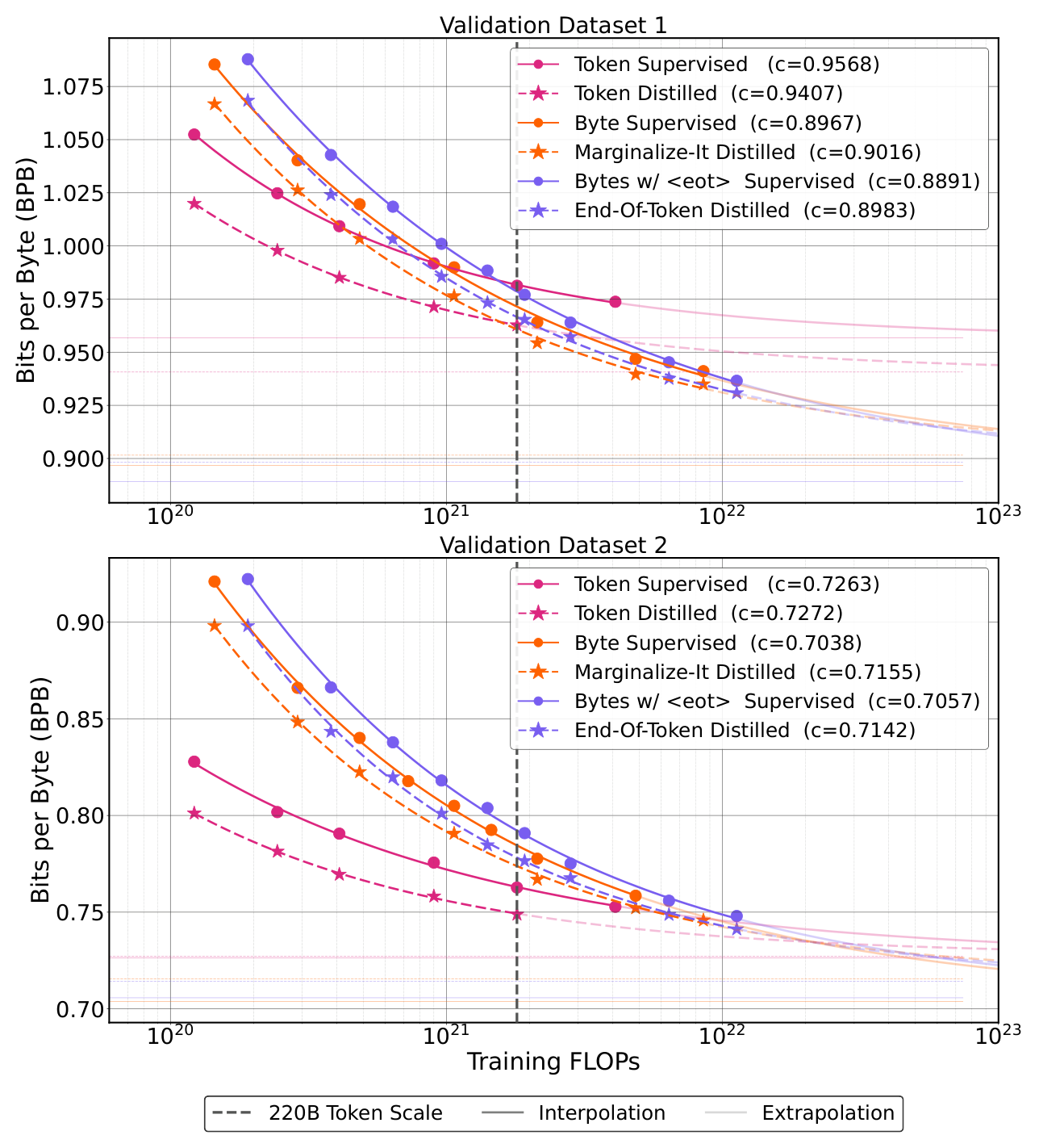
这是三组检查里最动摇结论的一组。换一个验证集后:
- 220B token 监督预算处,验证集 1 上其余五个模型 BPB 都更低;验证集 2 上只有蒸馏 token 模型更低。
- 两个验证集给出的渐近 BPB 完全不同(验证集 2 全部落在 0.70–0.75,验证集 1 在 0.88–0.96)。
- token 曲线与 byte 曲线的交叉点位置改变,Feather Plot 的形态也随之改变。
验证集 2 下的渐近准确率(Table 21):
| Model | $a^\star$ (1e-3) | $a^\star$ (4e-3) | $a^\star$ (8e-3) |
|---|---|---|---|
| Token Supervised | 43.6 | 47.9 | 47.6 |
| Token Distilled | 49.2 | 48.7 | 46.1 |
| Bytes Supervised | 47.4 | 50.5 | 47.5 |
| Marginalize-It Distilled | 48.1 | 48.9 | 46.5 |
Bytes w/ <eot> Supervised |
47.7 | 49.6 | 46.4 |
| End-Of-Token Distilled | 48.6 | 50.5 | 49.1 |
在验证集 2 上,4e-3 下 End-Of-Token Distilled(50.5)相对 Token Distilled(48.7)的优势从 +4.0 缩水到 +1.8,并且与 Bytes Supervised 打平;1e-3 下它甚至输给了 Token Distilled(48.6 vs 49.2)。 作者自己的结论是:"在拟合标度律时同时考虑多个验证集,可能有助于预测最终模型性能"——这实际上是对自己主结论强度的一次显著下修。
为什么相同的 BPB 可以对应不同的下游表现(附录 G)¶
这一节给出了全文最清晰的机制性解释,值得完整转述。
BPB 只是位置上目标 token 概率 $p_{\text{correct}}$ 的函数:每个位置的损失是 $-\log_2 p_{\text{correct}}$,一旦 $p_{\text{correct}}$ 固定,损失就固定。BPB 对剩余的 $1 - p_{\text{correct}}$ 质量如何分布在其他词表项上完全盲视。而下游准确率取决于目标是否是 arg max,也就是取决于整条分布的排序——而排序恰恰由 BPB 忽略的那部分残余质量决定。因此两个模型可以有完全相同的 BPB 却解码出完全不同的文本。
具体例子:目标句 Where's my tiramisu?,Llama3-8B tokenizer 切成 7 个 token、共 20 字节:
Where | 's | ␣my | ␣tir | am | isu | ?
设两个模型在每个位置都给正确 token 概率 $p_{\text{correct}} = 0.4$。于是每个位置损失 $-\log_2 0.4 = 1.32$ bit,总计 $7\times1.32 = 9.24$ bit:
$$\mathrm{BPB} = \frac{9.24}{20} = 0.462 \tag{10}$$
两个模型的 BPB 完全相同,差别只在剩下 0.6 的质量放在哪里(Table 24):
| Pos | Target | $p_{\text{correct}}$ | Model A distractors | A arg max | Model B distractors | B arg max |
|---|---|---|---|---|---|---|
| 1 | Where |
0.4 | There=0.35, When=0.25 |
Where ✓ |
There=0.5, When=0.1 |
There ✗ |
| 2 | 's |
0.4 | 're=0.3, 'd=0.3 |
's ✓ |
'd=0.5, 're=0.1 |
'd ✗ |
| 3 | ␣my |
0.4 | ␣your=0.35, ␣the=0.25 |
␣my ✓ |
␣be=0.5, ␣the=0.1 |
␣be ✗ |
| 4 | ␣tir |
0.4 | ␣bur=0.35, ␣piz=0.25 |
␣tir ✓ |
␣cal=0.5, ␣bur=0.1 |
␣cal ✗ |
| 5 | am |
0.4 | av=0.3, ig=0.3 |
am ✓ |
z=0.5, av=0.1 |
z ✗ |
| 6 | isu |
0.4 | ami=0.35, osa=0.25 |
isu ✓ |
one=0.5, osa=0.1 |
one ✗ |
| 7 | ? |
0.4 | .=0.35, !=0.25 |
? ✓ |
!=0.5, .=0.1 |
! ✗ |
Model A 每一步目标都排第一,贪心解码得到 Where's my tiramisu?——7/7 精确匹配。Model B 每一步都有一个 0.5 的干扰项压在 0.4 的目标之上,目标恒排第二,贪心解码拼出 There'd be calzone!——0/7。两个模型 BPB 都是 0.462,token 准确率却是 100% vs 0%。
等 BPB 只约束目标的概率值,不保证目标排第一。
核心贡献总结¶
- 单次前向的 token→byte logit 转换。提出
Marginalize-It(近似,对前缀匹配的 token 重归一化)与End-Of-Token(精确,向词表加<eot>吸收残余质量)两种方法,把 Hayase et al. (2025)、Phan et al. (2024) 需要多次教师前向的精确转换降到一次前向。 - 首个沿 tokenization × 训练目标两轴的大规模过训练标度研究。层参数对齐的 ≈1B decoder-only transformer,数据量最高到 1T bytes,三个学习率、两个验证集。
- 一个可操作的负面结论:BPB 不能跨 tokenization 方案与训练目标做公平比较;低 BPB 的模型可能下游更差。并给出机制解释(BPB 盲视残余质量的排序)。
- Feather Plot:一种把 iso-FLOP 点连线的可视化,用来读"在给定预算下哪条路线此刻领先"以及"何时发生交叉"。
- 效率结论:End-Of-Token 蒸馏达到 Token 蒸馏渐近性能只需 1/6 的独特文本、1/5 的 logit 存储,并且因为词表只有 ≈261,根本不需要 top-k 截断。
- 一个意外发现:每 ≈4.5 字节插一个
<eot>带来的 ≈30.94% 额外算力本身就抬高了渐近性能——这是独立于"分布保真"的第二重收益机制。
与已归档相关工作的对比¶
Compute Optimal Tokenization Compute Optimal Tokenization(FAIR at Meta + University of Washington, 2026-05-02)¶
关系:显式引用但原文未展开对比(related work 仅一句"analyze the impact of data compression on scaling laws")· 已加载对方精读
- 共同关注的问题:两篇都在说同一件事——tokenization 粒度是 LLM 标度律里一个长期被隐藏的自由变量,而既有的 Chinchilla 式结论("20 token / 参数")其实是 BPE 这一个特定 tokenizer 的副产品。两篇都放弃 token 级 loss,改用 bits-per-byte 作为跨 tokenizer 的不变度量,理由完全一致:byte 才是信息量的物理单位。两篇共享作者(Limisiewicz、Pagnoni、Iyer、Lewis、Zettlemoyer),可以看作同一条研究线的前后两步。
- 相近的技术骨架:都是"大规模受控网格 → 拟合幂律 → 外推出可操作的处方"。Compute Optimal Tokenization 训练 988 个 BLT + 320 个 subword 模型,扫 (compute, 压缩率 $T$, 语言) 三维网格,拟合 $B^\star(C,T) \cong B_0 C^\alpha T^\beta$;本文训练 6 个场景 × 多个数据规模 × 3 个学习率,拟合 $y = bx^a + c$ 与 $z(y) = \epsilon - ke^{-\gamma y}$ 两层标度律。
- 结论上的相互印证:Compute Optimal Tokenization 的 Finding 是"最优压缩率随算力预算下降——更大的训练预算反而应当用更细粒度的 tokenizer",并把 Chinchilla 推广为"~60 bytes/param"。本文正是这条结论在极限处(压缩率 $T = 1$,即纯 byte)的实例化验证:算力足够大时 byte 模型的渐近 BPB 与渐近准确率都超过 BPE 模型。本文的 Table 3(每 token 总 FLOPs 越高、渐近 BPB 越低)与前者"最优 $\rho^\star \approx 60$ bytes/param 跨压缩率近似恒定"是同一现象的两种测法。
- 本文的差异与推进:(i) 前者只扫监督预训练,本文加上训练目标这第二根轴,并发现两根轴会交互(Table 4/14 显示同一 tokenization 下监督与蒸馏的 $\epsilon,k,\gamma$ 差异显著);(ii) 前者停在 validation loss,本文把链条延长到下游 benchmark,并因此发现了前者看不到的现象——低 BPB 不蕴含下游更好;(iii) 前者用 BLT 的 entropy 阈值平滑扫压缩率,本文则在纯 byte 一端引入
<eot>,把"每字节算力"当成可调旋钮(4.5 → 5.5 单元/token)。 - 可比的方法/实验差异:前者的模型规模从 50M 到 7B、算力 $5\times10^{18}$–$2\times10^{21}$ FLOPs,走的是 IsoFLOP 抛物线求最优点;本文固定 ≈1B 层参数、沿过训练方向扫数据量到 1T bytes,走的是渐近项外推。两者的方法论风险互补:IsoFLOP 拟合依赖每个预算的网格密度,渐近外推则依赖幂律尾部——本文的 LOO 分析显示 byte 曲线的 $c$ 散布明显大于 token 曲线(0.0098–0.0240 vs 0.0025–0.0050),这正是前者用 IsoFLOP 能规避的不确定性来源。
SMELT SMELT: Scaling Laws for Compute-Matched MoE Looped Transformers(Tsinghua + ByteDance Seed + M-A-P + TokenWave.AI, 2026-09-01)¶
关系:独立并发(本文未引用 SMELT,SMELT 也未引用本文;两篇相隔 10 天,殊途同归)· 已加载对方精读
- 共同关注的问题:两篇的 root cause 完全同构——当一个架构改动同时改变参数量和每 token 算力时,"匹配哪个预算"决定了结论是什么,而文献长期只匹配参数量、把额外 FLOPs 当成架构胜利记账。SMELT 把这句话写成了一句话:"a fraction of the parameter count is not a fraction of the cost." 本文遇到的是完全对称的问题:Token-1B 总参数 1.81B、byte 模型只有 1.28B,但 byte 模型每个 BPE token 要花 4.5–5.5 倍的 FLOPs。两篇都拒绝把这个不对称扫到地毯下。
- 相近的技术骨架:都是"先把预算口径拆清楚 → 在拆清楚的口径下跑跨规模标度阶梯 → 为每种架构各自拟合一条独立的标度面 → 把点观测升级成可外推的断言"。SMELT 用 MoE 同时锁死 per-token FLOPs、总参数量、KV cache 三个预算;本文则锁死"层参数量",并把泄漏出去的那部分算力(FLOPs/unit × units/token)明确列成 Table 3 的一列。
- 本文的差异与推进:结论方向恰好相反,而且这个相反是实质性的。SMELT 的立场是"扣掉额外算力之后循环还有没有优势",答案是有但只值 6.8–18.0% 的 FLOPs;本文的立场是"额外算力本身就是这个方案的一部分收益"——Table 3 显示渐近 BPB 随 Total FLOPs Per Token 单调下降,作者据此把
<eot>的 ≈30.94% 额外算力当成设计选择而非记账漏洞来解释("unintended but remarkable consequence")。换句话说,SMELT 要求把算力从架构功劳里减出去,本文则论证在固定数据量下多花算力是一条独立可用的标度轴。 - 可比的方法/实验差异:SMELT 在 100M–1.6B active(最高 54B 非嵌入参数)的 4×4 网格上拟合 Chinchilla 式曲面,并直接给出前沿指数 $\gamma$ 从 0.237 升到 0.250;本文固定 ≈1B 层参数、只沿数据量方向扫,靠渐近项 $c$ 和指数外推。SMELT 对本文最尖锐的提醒是:本文的
End-Of-Token DistilledvsToken Distilled比较不是 FLOP-matched 的(每 token 6.35× 的算力差),如果按 SMELT 的三重匹配口径重做,+4.0% 里有多少属于"分布保真"、多少属于"多花算力"会被彻底分开——而本文只在Bytes SupervisedvsBytes w/ <eot> Supervised这一对上做了近似的分离(51.2 → 51.6,即约 +0.4 归给算力),暗示剩下的大部分归给蒸馏精确性,但这个分解没有被显式验证。
On the Equivalence Between Auto-Regressive Next Token Prediction and Full-Item-Vocabulary Maximum Likelihood Estimation in Generative Recommendation--A Short Note AR-NTP 与 FV-MLE 的等价性(Kuaishou Technology, 2026-04-17)¶
关系:独立并发(本文未引用,对方也不在本文视野内;跨领域殊途同归)· 已加载对方精读
- 共同关注的问题:把一个粗粒度符号拆成一串细粒度符号时,诱导出的分布还是不是原来那个分布? Kuaishou 这篇短理论备忘问的是"$k$-token 自回归 NTP 到底在拟合什么分布",本文问的是"BPE token 分布摊到 byte 位置上还剩多少"。两者指向同一个 root cause:分解的合法序列空间与原符号空间之间必须是双射(bijection),否则分区函数对不上。
- 相近的技术骨架:两篇的核心论证都落在分区函数(归一化常数)的等价性上。Kuaishou 的 Theorem 1 证明 $\prod_{m=1}^{k} Z_m(\cdot) = \sum_{i\in\mathcal{V}}\exp(\ell(h,i)) = Z_{\text{full}}(h)$,前提恰恰是存在双射 $\Phi: \mathcal{V}\leftrightarrow\mathcal{S}$;并明确指出"如果 token-item 映射不是 bijection(如码本坍缩、碰撞),则 $\prod_m Z_m$ 会多数出一些非法序列,从而严格大于 $Z_{\text{full}}$——此时 AR-NTP 就是 FV-MLE 的有偏逼近"。本文的
Marginalize-It正是这个有偏逼近的一个真实实例:BPE 的字节分解不是前缀无歧义的(is既是完整 token 又是isu/isk的前缀),于是"长度 ≥ k+1"这个筛选条件会静默丢掉恰好在此结束的路径,归一化就错了。 - 本文的差异与推进:Kuaishou 的贡献是从证明侧给出条件(双射成立则等价,不成立则有偏),停在那里;本文的贡献是从构造侧给出修复——加一个
<eot>让is<eot>的字节长度变成 3,从而使 byte 序列空间重新变成前缀无歧义的,双射条件被人为恢复,等价性随之成立(本文附录 F.2 情形 III/IV 逐一验证)。两篇合起来读,<eot>就是"把一个非双射的分词方案强行补成双射"的最小构造,而 Kuaishou 的定理恰好解释了为什么补完之后精确性会自动成立。 - 可比的方法/实验差异:Kuaishou 的动机是工业生成式推荐的 SID 分词(级联 RQ-VAE / 并行 OPQ),复杂度关切是把 $O(V)$($V\sim10^6$–$10^9$)全词表 softmax 分解成 $k$ 次 $O(V_m)$ 小 codebook softmax;本文的动机是 LLM 离线蒸馏,复杂度关切是把 $|V| = 128{,}256$ 的 logit 存储压到 260 维。两者的"为什么要拆"完全不同(一个为了 softmax 可算,一个为了 logit 可存),但"拆完还对不对"这个问题的数学结构是同一个。Kuaishou 侧的现实风险是 SID 碰撞破坏双射,本文侧的现实风险是 BPE 前缀歧义破坏双射——两边的补救思路(QuaSID/AdaSID 的碰撞缓解 vs 本文的
<eot>)本质上都是在恢复双射。
讨论与局限性¶
作者自己的讨论¶
Marginalize-It vs End-Of-Token。Marginalize-It 尽管是近似,渐近上仍然打败了 token 蒸馏基线。End-Of-Token 有两项优势:(1) 精确保留教师分布;(2) 以每单位数据多花 ≈30.94% 算力为代价,抬高了 End-Of-Token-1B 监督基线自身的渐近性能。这两项叠加,使 End-Of-Token 蒸馏在下游任务上渐近超过其余五个配置。
<eot> 对幂律的作用。仅仅是平均每 ≈4.5 字节加一个 <eot>,就改变了幂律系数(Table 3);监督版的 End-Of-Token-1B 也比 Bytes-1B 基线有更好的渐近下游表现。作者认为这"开启了许多令人兴奋的未来方向"。
推理成本(作者主动承认的最大短板)。标度律说明把 Llama3-8B 蒸馏进 1.28B 的 End-Of-Token-1B 比蒸馏进 1.81B 的 Token-1B 渐近更好,但 End-Of-Token-1B 在推理时仍然显著更贵(序列长度 11264 vs 2048)。"在匹配推理成本的前提下,把更大的 Token-1B 与更小的 End-Of-Token-1B 比较,才能揭示蒸馏 End-Of-Token transformer 是否在推理侧也高效——这超出本研究范围。"
BPB 与 benchmark 表现的错位。作者指出这不是孤例:不同优化器(Zhang et al. 2026)、不同数据分布(Gadre et al. 2024)、长上下文(Fang et al. 2025)、byte 建模(Lee et al. 2026)以及理论分析(Liu et al. 2023;Veličković et al. 2026)都观察到同样现象。本文的增量是识别出训练目标与tokenization 方案这两个新的触发条件。
未来工作:(1) 加入稀疏性作为第三根轴(MoE);(2) 本研究固定 ≈1.28B 层参数,且部分较大的 run 出现了 epoch(数据重复),未来应扩大模型规模与数据量;(3) 扩展到更多 benchmark;(4) 把大 byte transformer 蒸馏进小 byte transformer 的训练动力学仍是开放问题。
我的补充判断¶
值得借鉴的设计:
<eot>这个构造极其廉价且收益是双重的。它既修复了分布保真(把"token 在此结束"这条路径显式化),又顺带成为一条可调的"每字节算力"旋钮。对推荐系统而言,这个思路直接可迁移:SID 分词里的码本碰撞本质上也是"双射被破坏",而本文提示的补救方向是"加一个显式终止符号把歧义路径拆开",而不是像 QuaSID/AdaSID 那样在码本训练阶段做碰撞缓解。- Feather Plot 是一个被低估的工具。它解决的是标度律实践中最实际的问题——不是"谁最终赢",而是"在我此刻的预算下,谁赢"。任何要在多条技术路线间做预算分配的团队都能直接复用。
- Table 3 的呈现方式(把 FLOPs/unit、units/token、Total FLOPs/token 三列并排,再对齐渐近 BPB)是处理"参数匹配 ≠ 算力匹配"这类比较的好范式。
局限与争议:
- 几乎所有 headline 数字都是外推,而实测几乎持平。Table 18 里
End-Of-Token Distilled44.6 vsToken Distilled44.4——0.2 个点。"+4.0%"、"超过 Gemma 2B 2.1%"全部来自把两层拟合(BPB 幂律 + 误差指数律)串联后推到无限算力。两层拟合的误差会相乘,而作者只对第一层做了 LOO 与加权敏感性分析,第二层(式 8 的 $\epsilon, k, \gamma$)完全没有做不确定度分析。考虑到 $k$ 的量级在 185–1292 之间横跳、$\gamma$ 在 7.18–9.35 之间,$e^{-\gamma c}$ 这一项对 $c$ 的微小偏移极度敏感——Bytes w/ <eot> Supervised的 $k=185.6,\gamma=7.18$ 与Bytes Supervised的 $k=1231.1,\gamma=9.35$ 差了近 7 倍,却要用来支撑 51.2 vs 51.6 这样 0.4 个点的比较。 - 验证集 2 的结果实质上削弱了主结论,却只被放在附录。4e-3 下优势从 +4.0 缩到 +1.8 并与
Bytes Supervised打平,1e-3 下甚至反输给Token Distilled。作者的措辞是"考虑多个验证集可能有帮助",但更诚实的表述应当是"主结论的量级依赖于验证集选择"。 - 比较不是 FLOP-matched 的(见与 SMELT 的对比)。层参数对齐是一个有用的控制,但 End-Of-Token-1B 每 BPE token 花 $51.92\times10^9$ FLOPs,Token-1B 只花 $8.18\times10^9$——6.35 倍。论文把这解释成"byte 模型数据效率高"(用更少的数据达到同样性能),但从算力账本看它是"用更多算力换更少数据"。在数据不是瓶颈的场景里,这个交易是亏的。
- 推理成本是结构性的、不是工程可优化的。序列长度 2048 → 11264 意味着 attention 的 KV cache 和长上下文成本都成比例上升。作者把它列为 future work,但这恰恰是决定这条路线能否落地的那个变量——一个渐近上强 4% 但推理贵 5 倍的模型,在任何有 SLA 的系统里都不会被采纳。
Token Distilled只训到 220B token,其余配置到 500B–880B。这个不对称虽然本身就是"token logit 存储贵"的证据,但它同时让 Table 18 的实测比较不完全对等——如果 token 蒸馏也能训到 880B,44.4 这个数会涨多少是未知的,而 Figure 4 显示 token 曲线在 220B 附近确实还没完全平。- 较大 run 出现 epoch(数据重复)被一笔带过。数据重复会系统性地压低 validation BPB 的改善速度(见 Prescriptive Scaling Laws for Data Constrained Training 的 overfitting 惩罚项),而这恰好发生在外推最依赖的曲线尾部。这是对渐近项 $c$ 最危险的一类污染,论文没有量化它。
对推荐系统方向的启示(本文是纯 LLM 工作,但有可迁移点):
- 离线蒸馏的存储墙在推荐里同样存在。工业排序模型的 item 词表动辄 $10^8$–$10^9$,若要做 logit 级蒸馏,top-k 截断是必然的。本文的思路提示了一条替代路径:把学生放到一个更细粒度(因而词表更小)的符号空间上,用一个显式终止符恢复双射——这与 On the Equivalence Between Auto-Regressive Next Token Prediction and Full-Item-Vocabulary Maximum Likelihood Estimation in Generative Recommendation--A Short Note 的定理、以及 SID 领域正在做的碰撞缓解是同一件事的三个面。
- "BPB 更低不代表模型更好"在推荐里的对应物是"离线 AUC/NDCG 更高不代表线上更好",而本文给出了这个现象的一个可迁移的机制解释:损失只约束正样本的概率值,不约束负样本之间的排序,而线上指标由完整排序决定。这比"离线线上不一致"这句口号要精确得多。