AIR-MoE:用自适应倒排索引把"细粒度 MoE"的路由开销摊掉
研究动机与背景
细粒度 MoE 的"路由税"
Mixture-of-Experts (MoE) 通过对每个 token 只激活 $K$ 个专家来扩展 Transformer 容量而不显著增加计算量。给定 token 表示 $\mathbf{h}\in\mathbb{R}^d$、专家集合 $\{\mathrm{FFN}_\phi^{(e)}\}_{e=1}^E$ 与可学习专家中心 $\mathbf{w}_e\in\mathbb{R}^d$,标准 sparse MoE 写作:
$$ \mathrm{MoE}(\mathbf{h}) := \sum_{e\in\mathrm{TopK}\{\boldsymbol{\gamma}(\mathbf{h})\}} \gamma_e(\mathbf{h})\,\mathrm{FFN}_\phi^{(e)}(\mathbf{h}),\tag{1} $$
其中 $\gamma_e(\mathbf{h}) = \mathrm{softmax}(z_e(\mathbf{h}))$,$z_e(\mathbf{h}) := \langle\mathbf{w}_e,\mathbf{h}\rangle$。
Krajewski 等 (2024) 拟合的 scaling law 指出,专家越细粒度(每个专家越小、专家数越多)模型性能越好:
$$ \mathcal{L}(Q) = \frac{a}{Q^b} + c,\quad Q := \frac{d_{\mathrm{standard}}}{d_{\mathrm{expert}}}.\tag{3} $$
但当 $E$ 增长到几万乃至上百万级别时,路由本身要做 $E$ 次内积 $\langle\mathbf{w}_e,\mathbf{h}\rangle$,路由 FLOPs 变成主导项——这就是论文里反复强调的"granular MoE 实际不可训"的根因。在 MIPS 文献中这是经典的 maximum inner product search 问题,但已有的 ANN 解法没法直接搬到端到端可训练的 MoE 路由器里。
已有方案的不足
论文把先前路线分成三类,并指出共同的代价:
- Hierarchical / Hash MoE(Shazeer 2017、Roller 2021、Nogueira Dos Santos 2024):把专家按预定义层级或哈希桶分组,路由时只在选中的小组内取 top-$K$。Clark et al. (2022)、Dikkala et al. (2023) 已实证 hash 结构会限制表达能力。
- PEER(He 2024,Mixture of a Million Experts):把每个专家中心分解成两个 prototype 的笛卡尔积,路由从 $\mathcal{O}(SEd)$ 降到 $\mathcal{O}(Sd(\sqrt{E}+K^2))$。代价是给专家中心 $\mathbf{W}$ 强加结构约束,并且复杂度在 active experts 数 $k$ 上是二次的,必须把 MoE 改成多 head 才能补回来。
- VQ for MoE(Do et al. 2024):仅用 VQ 编码 token 表示后再打分,并不做 retrieval index,因此计算开销没降下来。
因此作者的目标很明确:做一个"几乎不改 MoE 架构"的 drop-in router,既不限制专家中心的参数空间,又能把 $E$ 大到几十万级别后的路由代价稳稳压住。
核心方法:AIR-MoE 总览
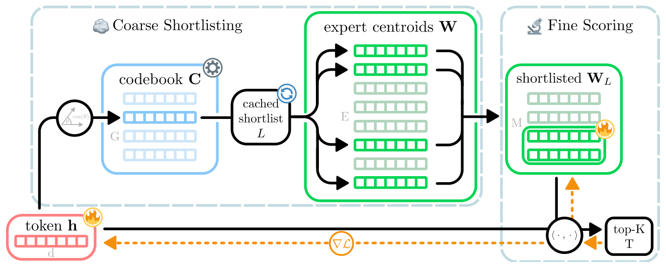
灵感来自经典的 Inverted File Index (IVF):先用一个粗粒度 quantizer 把查询定位到一个 cell,再在该 cell 的"posting list"里做精确打分。AIR-MoE 把这套思路端到端地塞进可训练 MoE:
- 粗筛 (Coarse Shortlisting):把 token $\mathbf{h}$ 通过一个尺寸 $G\ll E$ 的 codebook $\mathbf{C}=\{\mathbf{c}_g\}_{g=1}^G$ 量化到最近的 codeword,每个 codeword 维护一个预先打好的"专家短名单" $L(\mathbf{c}_g)$(top-$M$ experts under $\langle\mathbf{c}_g,\mathbf{w}_e\rangle$)。
- 精打 (Fine Scoring):在 $L(\mathbf{c}_{g_s})$ 内对 token 与候选专家做精确内积,再在其中取 top-$K$。
形成包含层级 $T\subset L\subset[E]$(公式 4),可以理解为对 exact top-$K$ 路由的一个 FLOP-efficient 近似。
前向流程(Algorithm 1)
Input: token batch H={h_s}_{s=1..S}, codebook C={c_g}_{g=1..G},
       expert centroids W, shortlist size M, top-K, jitter ε>0
Output: top-K expert indices T_s and scores z_s

1. w_e ← Π_{S^d}(w_e), ∀e∈[E]                  # normalize expert centroids
2. for s=1..S:
3.     g_s ← argmax_{g∈[G]} sim_cos(h_s, c_g)
4. if shortlist cache invalid:
5.     for g=1..G:
6.         η_1 ~ N(0, ε²I)
7.         L_g ← TopM_{e∈[E]} (⟨c_g, w_e⟩ + η_1)
9. for s=1..S:
10.    η_2 ~ N(0, ε²I)
11.    T_s, z_s ← TopK_{e∈L_{g_s}} (⟨h_s, w_e⟩ + η_2)
13. return {T_s, z_s}_{s=1..S}
几个关键设计:
- Shortlist cache:codeword→shortlist 只在 codebook 或 expert centroids 更新后(即一个 optimizer step 之后)重算一次,因此 $\mathcal{O}(EGd)$ 的开销摊给整个 effective batch(micro-batch × gradient accumulation steps)。在大有效批的训练下,单 token 的均摊路由代价与 $E$ 无关。
- Cosine 相似度:codebook 用 cosine(line 3),shortlist 构造也是基于 unit-sphere 的内积,因此 line 1 把所有专家中心投影到 $\mathbb{S}^d$。投影也是 Prop. 1 中"路由质量下界"的关键前提。
- 双 jitter:line 6 与 line 10 各加一次 Gaussian 噪声 $\eta\sim\mathcal{N}(0,\epsilon^2 I)$,鼓励 shortlist 与 expert 选择的探索性,避免 codebook 收敛到死循环。
- Switch-style load balancing:另外加 Fedus 等 (2022) 的 load-balancing loss 防止专家饥饿。
粗筛细节
对一个 batch $\mathbf{H}=\{\mathbf{h}_s\}_{s=1}^S$,每个 token 通过 cosine 相似度落到 codeword 上:
$$ g_s := \arg\max_{g\in[G]} \mathrm{sim}_{\cos}(\mathbf{h}_s, \mathbf{c}_g),\quad \mathrm{sim}_{\cos}(\mathbf{x},\mathbf{y}) := \frac{\langle\mathbf{x},\mathbf{y}\rangle}{\|\mathbf{x}\|\|\mathbf{y}\|}.\tag{5} $$
assigned codeword 记为 $c(\mathbf{h}_s):=\mathbf{c}_{g_s}$。每个 codeword 持有一个长度 $M$ 的 expert shortlist $L(\mathbf{c}_g)$,按同样规则(cosine)选出,每个 optimizer step 后用最新的 $\{\mathbf{w}_e\}$ 全量扫一遍刷新。这套结构对应一个学习出来的 inverted file:codeword 是 coarse cell,shortlist 是 posting list。
训练:bi-level 优化
AIR-MoE 的关键创新之一是把 codebook 训练完全脱钩于其他模型参数:
| 部分 | 更新方式 |
|---|---|
| Token 表示 $\mathbf{H}$、专家中心 $\mathbf{W}$、Transformer 参数 | 标准下游 LM loss + 梯度反传(不经过量化阶段,不用 straight-through estimator) |
| Codebook $\mathbf{C}$ | gradient-free Adaptive Spherical K-Means(Algorithm 2) |
之所以能丢掉 STE,是因为 codebook 只在 shortlisting(line 7)里出现,参与 fine scoring(line 11)的是真正的 $\mathbf{h}, \mathbf{w}_e$;codebook 的"非可微"性质被设计成天然不需要传梯度。
Adaptive Spherical K-Means(Algorithm 2)
Input: H={h_s}_{s=1..S}, codebook C, decay γ∈[0,1),
       running counts n, running sums M, dead-code threshold τ
1. for s=1..S:
2.     h'_s ← Π_{S^d}(h_s)                       # normalize token state
3.     g_s ← argmax_{g∈[G]} sim_cos(h'_s, c_g)
4. for g=1..G:
5.     n_g^batch ← Σ_s 1[g_s==g]
6.     m_g^batch ← Σ_s 1[g_s==g]·h'_s
7.     n_g ← γ·n_g + (1-γ)·n_g^batch              # EMA counts
8.     m_g ← γ·m_g + (1-γ)·m_g^batch              # EMA sums
9.     if n_g < τ:
10.        u ~ Unif([S]); m_g ← h'_u; n_g ← 1     # reinit dead code
13.    c_g ← Π_{S^d}(m_g)                          # update & normalize
14. return C, n, m
三个互相补强的设计:
- Exponential Moving Average(lines 7-8,借鉴 Van Den Oord 2017 的 VQ-VAE EMA codebook):用 EMA 跟踪 token 表示空间的缓慢漂移——transformer 参数会持续更新,token 表示分布每个 step 都在挪。
- Spherical K-Means(lines 2, 13,Dhillon & Modha 2001):所有 token 与 codeword 都先投到单位球面再聚类。Lelu & Cadot (2019) 等已表明高维下球面聚类更稳。这一选择直接对应到 Prop. 1 中 $\|\mathbf{w}_e\|\le 1$ 的假设。
- Dead-code reinitialization(lines 9-12,Williams 2020):若某 codeword 的 EMA count 低于阈值 $\tau$,就用当前 batch 中随机一个 token 表示替换之,避免 codeword "饿死"。这与 sparse MoE 中的 dying expert 现象类似。
完整训练循环见 Algorithm 3:每个 step 先做一次 codebook EMA 更新(adaptive spherical k-means),然后做 codeword 分配 → 懒计算 shortlist cache → fine scoring → 算 LM loss + router loss → 反传更新 $\theta$ → 失效 shortlist cache 等待下次刷新。
理论:路由质量下界
Mass Recall 定义
定义在 token $\mathbf{h}$ 上的完整路由分布
$$ \pi_e(\mathbf{h}) := \frac{\exp\{z_e(\mathbf{h})\}}{\sum_{j=1}^E \exp\{z_j(\mathbf{h})\}},\quad e\in[E], $$
以及短名单内被保留的概率质量
$$ \mathrm{MassRecall}(\mathbf{h}) := \sum_{e\in L(c(\mathbf{h}))} \pi_e(\mathbf{h}). $$
直观上 mass recall 越大,shortlist 越能覆盖真正"重要"的专家。
Proposition 1(Routing Mass Preservation)
设 $\epsilon(\mathbf{h}) := \|\mathbf{h}-c(\mathbf{h})\|$(量化误差),$L(c(\mathbf{h}))$ 是 codeword 视角下 top-$M$ experts。则
$$ \mathrm{MassRecall}(\mathbf{h}) \ge \exp(-2\epsilon(\mathbf{h}))\,\rho_M(c(\mathbf{h})), $$
其中
$$ \rho_M(c(\mathbf{h})) := \sum_{e\in L(c(\mathbf{h}))}\pi_e(c(\mathbf{h})) $$
是 codeword 自己的 shortlist mass。
证明骨架(附录 B)
由 Cauchy-Schwarz 与 $\|\mathbf{w}_e\|\le 1$:
$$ |z_e(\mathbf{h}) - z_e(\mathbf{c})| = |\langle\mathbf{w}_e, \mathbf{h}-\mathbf{c}\rangle| \le \epsilon(\mathbf{h}). $$
于是 $z_e(\mathbf{h})\ge z_e(\mathbf{c})-\epsilon(\mathbf{h})$,$z_e(\mathbf{h})\le z_e(\mathbf{c})+\epsilon(\mathbf{h})$。指数化后
$$ \exp\{z_e(\mathbf{h})\} \ge \exp(-\epsilon)\exp\{z_e(\mathbf{c})\},\quad \exp\{z_e(\mathbf{h})\} \le \exp(\epsilon)\exp\{z_e(\mathbf{c})\}. $$
把上界用于分母、下界用于分子代入 mass recall 的定义并化简,即得 $\exp(-2\epsilon(\mathbf{h}))\rho_M(c(\mathbf{h}))$。
两层启示:
- 量化误差越小 → 下界越紧。这就是 codebook 必须"自适应"地跟踪表示分布的根因——表示在变,固定 codebook 的 $\epsilon$ 会越来越大。
- shortlist 越大 → $\rho_M$ 越大 → 下界越大,但代价是更多的 fine scoring FLOPs。
这给出了 $G$(codebook 大小,决定 $\epsilon$)和 $M$(shortlist 大小,决定 $\rho_M$)的可解释 trade-off,也说明了为什么 expert centroid 必须 unit-norm(line 1 的 $\Pi_{\mathbb{S}^d}$):没有这个归一化,Cauchy-Schwarz 就拿不到 $\epsilon$ 上界。
实验
数据集与基线
数据集:
- WikiText-103:~103M tokens(small/medium 规模),适合长依赖语言建模评测;
- C5(Common Crawl 派生):~87B tokens;
- OpenWebText2(The Pile 子集):~15-20B tokens。
Baseline router: 1. Std. Coarse:粗 MoE,$K=1$,专家少而大,作为 active-参数对齐的 baseline; 2. Std. Granular:粒度对齐的标准 granular MoE(exact top-$K$ over all $E$),FLOPs 上界,灰色; 3. PEER (He 2024):product-key router,$P=8$ heads; 4. Hierarchical MoE (Shazeer 2017):按预定义子组路由。
架构
LLaMA-3 tokenizer (vocab 128 256)、最大 seq len 2048、RoPE base $\theta=5\times 10^5$、GQA 4:1、tied embedding。三种规模:
| 超参 | Small | Medium | Large |
|---|---|---|---|
| $d_{\mathrm{model}}$ | 256 | 512 | 768 |
| $d_{\mathrm{ffn}}$ | 768 | 1536 | 2048 |
| Layers | 16 | 24 | 24 |
| Attn heads | 4 | 8 | 12 |
| KV heads | 1 | 2 | 4 |
| Total params | ≈61M | ≈0.27B | ≈0.45B |
所有模型用 65 536 个专家进行实验,active expert 数固定 $K=512$。优化器 AdamW($\beta_1=0.9, \beta_2=0.95$)、weight decay 0.1、grad clip 1.0、peak LR $3\times10^{-4}$、5% linear warmup、fp16。
AIR-MoE 全局超参(所有实验不调):$\gamma=0.95$(EMA decay),$\tau=1.0$(dead-code 阈值),$\lambda=5\times 10^{-5}$(load balancing 权重),$\epsilon=0.01$(jitter 方差)。
主实验:PPL × FLOPs trade-off(Table 1)
| Size | Method | WikiText-103 PPL ↓ | WikiText-103 FLOPs ↓ | C5 PPL ↓ | C5 FLOPs ↓ | OpenWebText2 PPL ↓ | OpenWebText2 FLOPs ↓ |
|---|---|---|---|---|---|---|---|
| Small | AIR | 21.82 | 324.1P | 131.81 | 625.5P | 32.14 | 505.0P |
| Small | PEER | 22.25 | 352.8P | 145.32 | 626.3P | 33.10 | 505.6P |
| Small | Hierarchical | 22.55 | 350.4P | 147.99 | 622.6P | 36.05 | 502.6P |
| Small | Std. Granular | 21.34 | 467.5P | 132.34 | 817.2P | 31.56 | 648.3P |
| Small | Std. Coarse | 23.84 | 342.5P | 151.99 | 611.7P | 36.05 | 493.9P |
| Medium | AIR | 18.62 | 755.9P | 30.39 | 4.1E | 20.51 | 3.6E |
| Medium | PEER | 18.71 | 751.0P | 31.60 | 4.1E | 21.30 | 3.5E |
| Medium | Hierarchical | 19.27 | 954.7P | 33.08 | 4.1E | 23.07 | 3.5E |
| Medium | Std. Coarse | 18.79 | 836.7P | 32.10 | 4.0E | 21.25 | 3.5E |
| Large | AIR | – | – | 41.25 | 14.3E | 16.65 | 11.2E |
| Large | PEER | – | – | 45.37 | 14.0E | 17.88 | 11.2E |
| Large | Hierarchical | – | – | 45.65 | 14.4E | 18.17 | 11.3E |
| Large | Std. Coarse | – | – | 43.13 | 13.2E | 16.98 | 11.3E |
Std. Granular 是 exact-routing 上界,灰色仅参考;WikiText-103 large 因严重过拟合被省略。
关键观察:
- Pareto 优势:在 5/8 个 (size, dataset) 配置下 AIR 取得最低 PPL;剩余几个 large/coarse 略胜处也只是 PPL 差距很小但 FLOPs 高得多。
- PPL 几乎贴近 exact:以 WikiText-103 small 为例,AIR 21.82 vs Std. Granular 21.34(差 0.48),但 FLOPs 324.1P vs 467.5P(省 31% router-included FLOPs)。
- 比 PEER 稳定占优:在所有规模与数据集上 AIR PPL 持续低于 PEER,差距随数据集和规模有所扩大(OpenWebText2 large: 16.65 vs 17.88)。
相对 PPL 改进图(Figure 2)
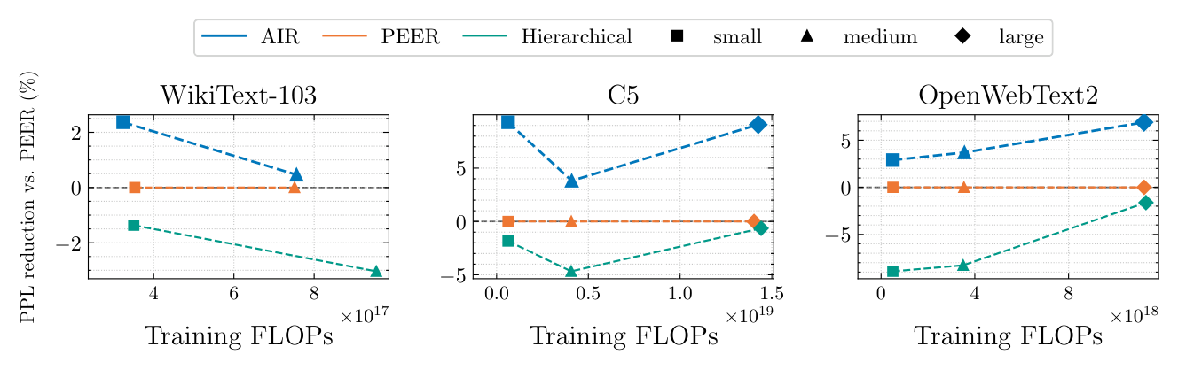
把 PEER 设为 0 基线,AIR 在三套数据集上的 PPL 相对降幅最高达约 10%,在 medium/large 规模尤其稳定。Hierarchical 几乎全程在负值线下面,说明硬分组的限制确实损害质量。
消融实验(Table 2)
WikiText-103 small 模型:
| Ablation | PPL ↓ | FLOPs ↓ | Dead Experts ↓ | Overlap ↑ | Entropy ↑ |
|---|---|---|---|---|---|
| AIR(完整) | 21.72 | 324.1P | 0.0% | 0.64 | 10.80 |
| Euclidean | 21.83 | 324.1P | 0.3% | 0.64 | 10.81 |
| Expert Choice | 22.77 | 357.5P | 78.6% | 0.74 | 9.53 |
| Missing Normalization | 21.96 | 324.1P | 0.7% | 0.66 | 10.73 |
| Static Code | 23.27 | 360.1P | 42.4% | 0.07 | 10.24 |
四个变体的解读:
- Euclidean assignment(去掉球面归一化、用欧氏距离做 k-means):PPL 仅微涨,但 dead expert 比例上升,说明 spherical 是更稳的高维聚类选择。
- Expert Choice gating (Zhou et al. 2022):即让专家自己挑 token、shortlist 外的 token 给 $-\infty$。Overlap 最高(0.74)但 78.6% dead experts,PPL 大涨——直接说明 overlap 不是 routing 质量的可靠 proxy,覆盖率才是。
- Missing Normalization(去掉 expert centroid 投影到 $\mathbb{S}^d$):PPL 微涨。这个变体也是 Prop. 1 假设破坏的实证。
- Static Code(codebook 用初始 token 表示固定不更新):PPL 23.27,dead expert 42.4%,直接论证了 adaptive codebook 的必要性——分布漂移会让固定 codebook 完全失配。
完整指标(Table 3,附录 F.1)
附录里把 Dead Experts 和 routing Entropy 一并列了:
- Dead expert 几乎为零:除了 OpenWebText2 small 上 1.4%、WikiText-103 small 上 0.1%,其余配置全是 0%。Hierarchical 也是 0%(强约束的副作用);
- Routing entropy 与 PEER 接近(约 9.5-10.8),略低于 hierarchical(hierarchical 因为分组天然分散,entropy 更高,但 PPL 更差);
- Std. Coarse 的 entropy 只有 ~4——粗粒度专家少,本来就分散不开。
专家使用分布(Figure 4)
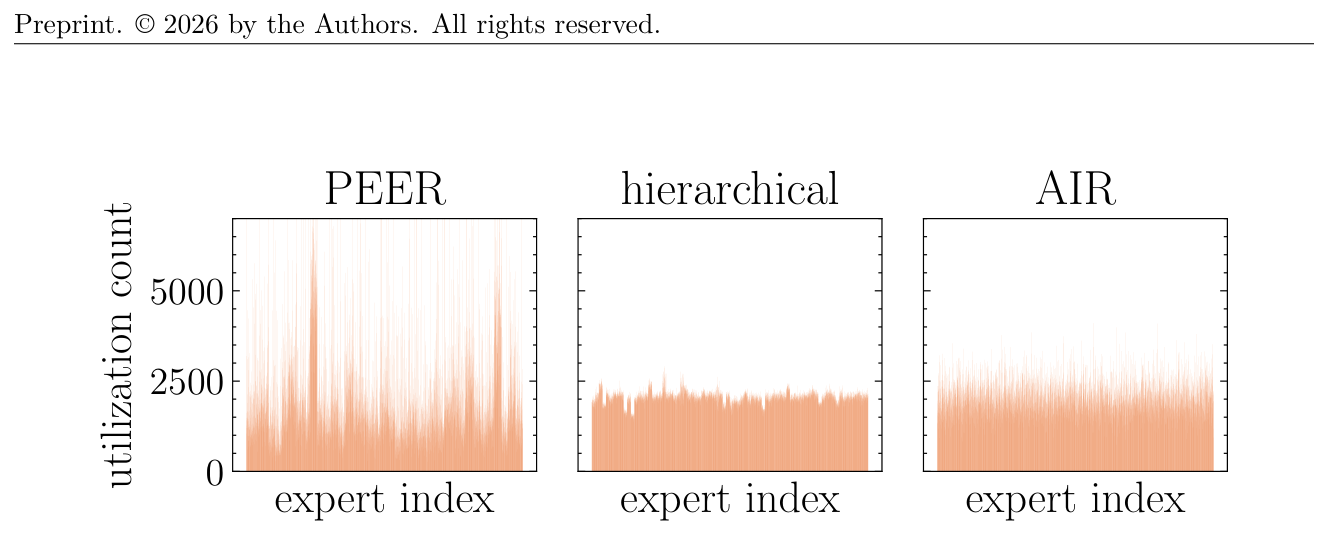
PEER 的产品键结构会引发显著的 hot expert 现象(少数索引使用频次高出几倍),而 hierarchical 的分组使专家利用率被人为拉平。AIR-MoE 既不强制平均也不长尾,而是在让 expert 之间形成自然分化的同时保持广泛覆盖。
讨论与局限性
Shortlist Updates 的 amortization 假设:每个 optimizer step 都要重算 $\mathcal{O}(EGd)$ 的 shortlist。当有效批大小较大时这部分被摊薄;但若工业训练把 micro-batch × accumulation 设得小(例如 RL fine-tune 阶段),这部分可能成为新瓶颈。论文坦承"FLOP 节省强依赖 $G, E, S$"。
Beyond Router FLOPs:作者明确指出,FLOPs 减少不等于 wall-clock 加速。granular MoE 的真正瓶颈往往是 memory traffic、indexing、不规则 expert call 等系统级开销(Lepikhin 2021、Fedus 2022)。AIR-MoE 当前的实现没有专门优化 kernel,硬件加速空间留给未来工作。
没尝试 dimensionality reduction:路由完全在原始 token space ($d$ 维) 进行;正交方向是先做学习的(Chi 2022)或随机的(Achlioptas 2001)降维再喂给 router。
核心贡献小结: 1. 把 IVF 思想 cleanly 移植到端到端 MoE 路由:codebook 学 coarse cell + 缓存 expert shortlist; 2. bi-level optimization——adaptive spherical k-means(gradient-free, EMA + reinit)独立训 codebook,token & expert centroids 完全跑标准梯度,无需 STE; 3. 给出 mass recall 的指数下界 $\exp(-2\epsilon)\rho_M$,直接联系 codebook 质量 ($\epsilon$) 和 shortlist 大小 ($M$) 两个旋钮; 4. 实验在 65k experts 设定下持续胜出 PEER 与 hierarchical,最高 10% PPL 改善,且 dead expert ≈ 0。
值得借鉴:bi-level(gradient-free codebook + gradient model parameters)的解耦设计,避免了所有 VQ 在端到端训练里挠头的 STE / commitment loss / codebook collapse 一系列问题;这种解耦思路(学一个不可微 index,retrieval 用 index、scoring 用真值)也可以复用到工业推荐里把 large user/item embedding tower 套上 inverted index。
主要争议 / 局限:
- 仅在 LM 任务上证明,未在 SFT、RLHF、code、math 等多任务上验证;
- 大模型规模 ≤0.45B,距 LLaMA-3 8B / 70B 还有数量级;
- 没有 wall-clock latency 数据,FLOP 优势能不能落到推理速度上仍是悬念;
- Codebook size $G$ 的选择机制论文没系统讨论(Tab/Fig 没扫 $G$)。